5.5: More Math Functions

Last updated
Save as PDF

Page ID: 14250

$ \newcommand{\vecs}[1]{\overset { \scriptstyle \rightharpoonup} {\mathbf{#1}} } $ $ \newcommand{\vecd}[1]{\overset{-\!-\!\rightharpoonup}{\vphantom{a}\smash {#1}}} $$\newcommand{\id}{\mathrm{id}}$ $ \newcommand{\Span}{\mathrm{span}}$ $ \newcommand{\kernel}{\mathrm{null}\,}$ $ \newcommand{\range}{\mathrm{range}\,}$ $ \newcommand{\RealPart}{\mathrm{Re}}$ $ \newcommand{\ImaginaryPart}{\mathrm{Im}}$ $ \newcommand{\Argument}{\mathrm{Arg}}$ $ \newcommand{\norm}[1]{\| #1 \|}$ $ \newcommand{\inner}[2]{\langle #1, #2 \rangle}$ $ \newcommand{\Span}{\mathrm{span}}$ $\newcommand{\id}{\mathrm{id}}$ $ \newcommand{\Span}{\mathrm{span}}$ $ \newcommand{\kernel}{\mathrm{null}\,}$ $ \newcommand{\range}{\mathrm{range}\,}$ $ \newcommand{\RealPart}{\mathrm{Re}}$ $ \newcommand{\ImaginaryPart}{\mathrm{Im}}$ $ \newcommand{\Argument}{\mathrm{Arg}}$ $ \newcommand{\norm}[1]{\| #1 \|}$ $ \newcommand{\inner}[2]{\langle #1, #2 \rangle}$ $ \newcommand{\Span}{\mathrm{span}}$$\newcommand{\AA}{\unicode[.8,0]{x212B}}$

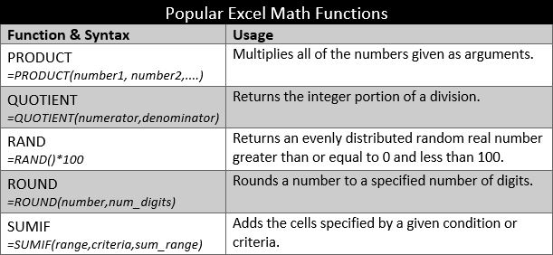
The most popular Excel function in the Math category is undoubtedly the SUM function. The Excel Math Functions perform many of the common mathematical calculations, including basic arithmetic, conditional sums & products, quotients, and rounding calculations. There are many more examples, but some of the more popular Math functions are identified in the table below. There are many variations of some of these functions to be found in the Insert Function window.

The first two functions from the table above are considered basic mathematical operations. Instead of multiplying two cells using the * operator, Excel users can opt to use the PRODUCT function. i.e. =PRODUCT(B2,B3) versus =B2*B3. The PRODUCT function is most useful when multiplying a series of cells. Ensure that the cells referenced contain numbers or dates. If the data referenced includes text, the PRODUCT function will return the #VALUE! error result.

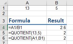
The QUOTIENT function is similar to the PRODUCT function, except instead of multiplying cells, it divides cell(s) by other cell(s) and returns a result in Integer format. An integer is a whole number, therefore it will not display the remainder typically generated in division calculations. The graphic at right illustrates the differences between using the divide operator and the QUOTIENT function. The numerator is the dividend and is the value before the forward slash (/). The denominator is the divisor, and is the value after the forward slash (/). In this example, A1 (or 13) is the dividend, and B1 (or 5) is the divisor.

An alternative to using the QUOTIENT function is to utilize the ROUND function or any of its related functions (ROUNDDOWN, ROUNDUP,MROUND).

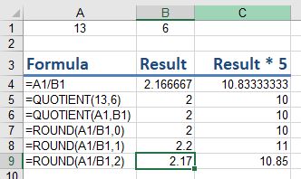
In the graphic above, a user could rewrite the formula in A4 as =ROUND(A1/B1,0) by using the ROUND function to get the similar results as the QUOTIENT functions. The difference is that the QUOTIENT result does not store any remainder amounts. As shown in the graphic at the right, using the ROUND function can yield significantly different results than using the QUOTIENT function, however, the user can control the level of detail desired in the calculation. Some users simply opt for the first scenario without using either functions. Instead, they utilize Excel’s formatting functionality to remove the displaying of decimals. Using the Decrease Decimal button from the ribbon on cell B4 can change the display to various results. However, the un-truncated/un-rounded result is still stored in the cell.

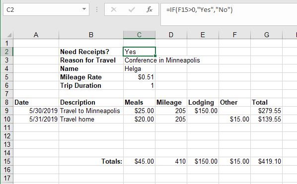
Practice 7: Expense Report

Create the a new worksheet with the following data from the image below:

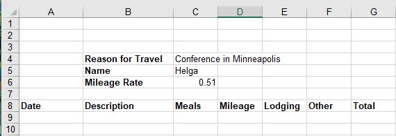
In row 9 enter the following data:
- Date: 5/30/2019
- Description: Travel to Minneapolis
- Meals: 25
- Mileage: 205
- Lodging: 150
- Other:
In cell G9 enter the following complex formula using relative and absolute cell references: =C9+(D9*$C$6)+E9+F9 (are the parenthesis necessary?)
Format columns C, E, F and G as Currency format with two decimals.
Enter the following in row 10:
- Date: 5/31/2019
- Description: Travel home
- Meals: 20
- Mileage: 205
- Lodging:
- Other: 15
Use the fill handle to copy the formula in G9 to G10.
Insert a new row below the Mileage Rate row, and in B6 enter the label: Trip Duration. (bold the label)
In cell C6 enter a formula that subtracts A9 from A10. Change the format of cell C6 to General.
In cell B15 enter the label: Totals: (right-align & bold this cell).
Select cells C15:G15 and click the AutoSum button. Change the format of D15 to General.
Enter the label: Need Receipts? in cell B2. (bold the label)
In cell C2, enter the following logical function: =IF(F15>0,”Yes”,”No”)
Save the file as Helga Expenses May2019. Your worksheet should resemble the following: