12.3.1: Query Performance Optimization

Query Performance Optimization

Working with large databases requires mindful SQL practices. Some general tips (reflecting standard optimization strategies) include:

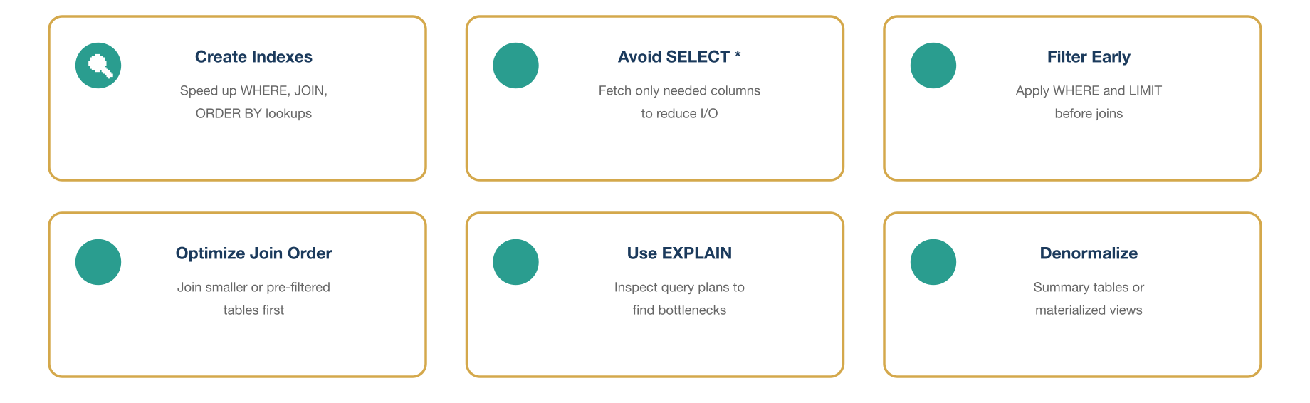
• Indexing: Create indexes on columns used in WHERE, JOIN, and ORDER BY clauses. Good indexes can speed lookups by orders of magnitude. For example, an index on customers.id speeds the join above.
• Avoid SELECT *: Only select needed columns. Fetching unnecessary fields wastes I/O.
• Proper Joins Order: Join smaller or filtered tables first if possible, to reduce intermediate result size.
• Use LIMIT or early filters: Filter data as early as possible. In analytics queries (e.g. dashboards), pagination or date limits help.
• Analyze/Explain: Use the database’s EXPLAIN feature to inspect query plans and identify bottlenecks. The database optimizer may reorder joins or choose indexes automatically, but understanding its plan can lead to rewriting queries for speed.
• Denormalization: In some analytics contexts, denormalizing schemas (e.g. summary tables) reduces expensive joins. For example, a star schema or materialized views can pre-aggregate data.
• CTE vs Subquery: Note that in many databases, non-recursive CTEs act like inline views. Their performance should match equivalent subqueries, but some systems differ (e.g. PostgreSQL can materialize CTEs).
• Window function cost: Use window functions judiciously; they may sort or partition large data. Sometimes a grouped aggregation is cheaper if you only need a single summary.

SQL performance tuning is a deep subject, but these principles help avoid common pitfalls. (The lecture notes on query optimization highlight similar points: understanding cardinality, minimizing I/O waste, and pushing computations to the database are key strategies.) For example, if many filters or transformations are needed, it is usually faster to do them in the database engine than fetching raw data and post-processing in another tool.

Figure \(\PageIndex{1}\): SQL Query Performance Optimization Strategies. An infographic summarizing six key optimization techniques -- indexing, selective column queries, join ordering, early filtering, EXPLAIN analysis, and denormalization -- with brief descriptions and impact indicators. (CC BY 4.0; Felix Amoruwa) Access to a detailed descripton of Figure \(\PageIndex{1}\)