10.4: Node Voltage Method
- Page ID
- 967
\( \newcommand{\vecs}[1]{\overset { \scriptstyle \rightharpoonup} {\mathbf{#1}} } \)
\( \newcommand{\vecd}[1]{\overset{-\!-\!\rightharpoonup}{\vphantom{a}\smash {#1}}} \)
\( \newcommand{\id}{\mathrm{id}}\) \( \newcommand{\Span}{\mathrm{span}}\)
( \newcommand{\kernel}{\mathrm{null}\,}\) \( \newcommand{\range}{\mathrm{range}\,}\)
\( \newcommand{\RealPart}{\mathrm{Re}}\) \( \newcommand{\ImaginaryPart}{\mathrm{Im}}\)
\( \newcommand{\Argument}{\mathrm{Arg}}\) \( \newcommand{\norm}[1]{\| #1 \|}\)
\( \newcommand{\inner}[2]{\langle #1, #2 \rangle}\)
\( \newcommand{\Span}{\mathrm{span}}\)
\( \newcommand{\id}{\mathrm{id}}\)
\( \newcommand{\Span}{\mathrm{span}}\)
\( \newcommand{\kernel}{\mathrm{null}\,}\)
\( \newcommand{\range}{\mathrm{range}\,}\)
\( \newcommand{\RealPart}{\mathrm{Re}}\)
\( \newcommand{\ImaginaryPart}{\mathrm{Im}}\)
\( \newcommand{\Argument}{\mathrm{Arg}}\)
\( \newcommand{\norm}[1]{\| #1 \|}\)
\( \newcommand{\inner}[2]{\langle #1, #2 \rangle}\)
\( \newcommand{\Span}{\mathrm{span}}\) \( \newcommand{\AA}{\unicode[.8,0]{x212B}}\)
\( \newcommand{\vectorA}[1]{\vec{#1}} % arrow\)
\( \newcommand{\vectorAt}[1]{\vec{\text{#1}}} % arrow\)
\( \newcommand{\vectorB}[1]{\overset { \scriptstyle \rightharpoonup} {\mathbf{#1}} } \)
\( \newcommand{\vectorC}[1]{\textbf{#1}} \)
\( \newcommand{\vectorD}[1]{\overrightarrow{#1}} \)
\( \newcommand{\vectorDt}[1]{\overrightarrow{\text{#1}}} \)
\( \newcommand{\vectE}[1]{\overset{-\!-\!\rightharpoonup}{\vphantom{a}\smash{\mathbf {#1}}}} \)
\( \newcommand{\vecs}[1]{\overset { \scriptstyle \rightharpoonup} {\mathbf{#1}} } \)
\( \newcommand{\vecd}[1]{\overset{-\!-\!\rightharpoonup}{\vphantom{a}\smash {#1}}} \)
\(\newcommand{\avec}{\mathbf a}\) \(\newcommand{\bvec}{\mathbf b}\) \(\newcommand{\cvec}{\mathbf c}\) \(\newcommand{\dvec}{\mathbf d}\) \(\newcommand{\dtil}{\widetilde{\mathbf d}}\) \(\newcommand{\evec}{\mathbf e}\) \(\newcommand{\fvec}{\mathbf f}\) \(\newcommand{\nvec}{\mathbf n}\) \(\newcommand{\pvec}{\mathbf p}\) \(\newcommand{\qvec}{\mathbf q}\) \(\newcommand{\svec}{\mathbf s}\) \(\newcommand{\tvec}{\mathbf t}\) \(\newcommand{\uvec}{\mathbf u}\) \(\newcommand{\vvec}{\mathbf v}\) \(\newcommand{\wvec}{\mathbf w}\) \(\newcommand{\xvec}{\mathbf x}\) \(\newcommand{\yvec}{\mathbf y}\) \(\newcommand{\zvec}{\mathbf z}\) \(\newcommand{\rvec}{\mathbf r}\) \(\newcommand{\mvec}{\mathbf m}\) \(\newcommand{\zerovec}{\mathbf 0}\) \(\newcommand{\onevec}{\mathbf 1}\) \(\newcommand{\real}{\mathbb R}\) \(\newcommand{\twovec}[2]{\left[\begin{array}{r}#1 \\ #2 \end{array}\right]}\) \(\newcommand{\ctwovec}[2]{\left[\begin{array}{c}#1 \\ #2 \end{array}\right]}\) \(\newcommand{\threevec}[3]{\left[\begin{array}{r}#1 \\ #2 \\ #3 \end{array}\right]}\) \(\newcommand{\cthreevec}[3]{\left[\begin{array}{c}#1 \\ #2 \\ #3 \end{array}\right]}\) \(\newcommand{\fourvec}[4]{\left[\begin{array}{r}#1 \\ #2 \\ #3 \\ #4 \end{array}\right]}\) \(\newcommand{\cfourvec}[4]{\left[\begin{array}{c}#1 \\ #2 \\ #3 \\ #4 \end{array}\right]}\) \(\newcommand{\fivevec}[5]{\left[\begin{array}{r}#1 \\ #2 \\ #3 \\ #4 \\ #5 \\ \end{array}\right]}\) \(\newcommand{\cfivevec}[5]{\left[\begin{array}{c}#1 \\ #2 \\ #3 \\ #4 \\ #5 \\ \end{array}\right]}\) \(\newcommand{\mattwo}[4]{\left[\begin{array}{rr}#1 \amp #2 \\ #3 \amp #4 \\ \end{array}\right]}\) \(\newcommand{\laspan}[1]{\text{Span}\{#1\}}\) \(\newcommand{\bcal}{\cal B}\) \(\newcommand{\ccal}{\cal C}\) \(\newcommand{\scal}{\cal S}\) \(\newcommand{\wcal}{\cal W}\) \(\newcommand{\ecal}{\cal E}\) \(\newcommand{\coords}[2]{\left\{#1\right\}_{#2}}\) \(\newcommand{\gray}[1]{\color{gray}{#1}}\) \(\newcommand{\lgray}[1]{\color{lightgray}{#1}}\) \(\newcommand{\rank}{\operatorname{rank}}\) \(\newcommand{\row}{\text{Row}}\) \(\newcommand{\col}{\text{Col}}\) \(\renewcommand{\row}{\text{Row}}\) \(\newcommand{\nul}{\text{Nul}}\) \(\newcommand{\var}{\text{Var}}\) \(\newcommand{\corr}{\text{corr}}\) \(\newcommand{\len}[1]{\left|#1\right|}\) \(\newcommand{\bbar}{\overline{\bvec}}\) \(\newcommand{\bhat}{\widehat{\bvec}}\) \(\newcommand{\bperp}{\bvec^\perp}\) \(\newcommand{\xhat}{\widehat{\xvec}}\) \(\newcommand{\vhat}{\widehat{\vvec}}\) \(\newcommand{\uhat}{\widehat{\uvec}}\) \(\newcommand{\what}{\widehat{\wvec}}\) \(\newcommand{\Sighat}{\widehat{\Sigma}}\) \(\newcommand{\lt}{<}\) \(\newcommand{\gt}{>}\) \(\newcommand{\amp}{&}\) \(\definecolor{fillinmathshade}{gray}{0.9}\)Method for Node Voltage Calculation
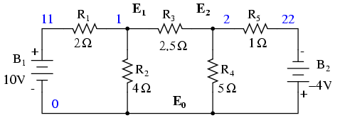
We start with a circuit having conventional voltage sources. A common node E0 is chosen as a reference point. The node voltages E1 and E2 are calculated with respect to this point.

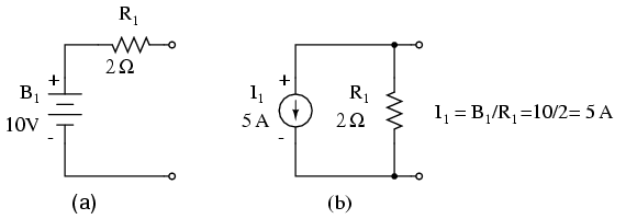
A voltage source in series with a resistance must be replaced by an equivalent current source in parallel with the resistance. We will write KCL equations for each node. The right hand side of the equation is the value of the current source feeding the node.

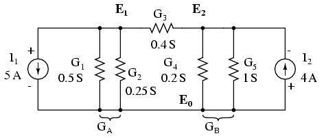
Replacing voltage sources and associated series resistors with equivalent current sources and parallel resistors yields the modified circuit. Substitute resistor conductances in siemens for resistance in ohms.

The parallel conductances (resistors) may be combined by addition of the conductances. Though, we will not redraw the circuit. The circuit is ready for application of the node voltage method.
Deriving a general node voltage method, we write a pair of KCL equations in terms of unknown node voltages V1 and V2 this one time. We do this to illustrate a pattern for writing equations by inspection.
The coefficients of the last pair of equations above have been rearranged to show a pattern. The sum of conductances connected to the first node is the positive coefficient of the first voltage in equation (1). The sum of conductances connected to the second node is the positive coefficient of the second voltage in equation (2). The other coefficients are negative, representing conductances between nodes. For both equations, the right hand side is equal to the respective current source connected to the node. This pattern allows us to quickly write the equations by inspection. This leads to a set of rules for the node voltage method of analysis.
Node Voltage Rules:
- Convert voltage sources in series with a resistor to an equivalent current source with the resistor in parallel.
- Change resistor values to conductances.
- Select a reference node(E0)
- Assign unknown voltages (E1)(E2) ... (EN)to remaining nodes.
- Write a KCL equation for each node 1,2, ... N. The positive coefficient of the first voltage in the first equation is the sum of conductances connected to the node. The coefficient for the second voltage in the second equation is the sum of conductances connected to that node. Repeat for coefficient of third voltage, third equation, and other equations. These coefficients fall on a diagonal.
- All other coefficients for all equations are negative, representing conductances between nodes. The first equation, second coefficient is the conductance from node 1 to node 2, the third coefficient is the conductance from node 1 to node 3. Fill in negative coefficients for other equations.
- The right hand side of the equations is the current source connected to the respective nodes.
- Solve system of equations for unknown node voltages.
Example: Set up the equations and solve for the node voltages using the numerical values in the above figure.
Solution:
The solution of two equations can be performed with a calculator, or with octave (not shown).[octav] The solution is verified with SPICE based on the original schematic diagram with voltage sources.[spi] .Though, the circuit with the current sources could have been simulated.
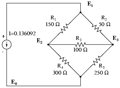
One more example. This one has three nodes. We do not list the conductances on the schematic diagram. However, G1 = 1/R1, etc.

There are three nodes to write equations for by inspection. Note that the coefficients are positive for equation (1) E1, equation (2) E2, and equation (3) E3. These are the sums of all conductances connected to the nodes. All other coefficients are negative, representing a conductance between nodes. The right hand side of the equations is the associated current source, 0.136092 A for the only current source at node 1. The other equations are zero on the right hand side for lack of current sources. We are too lazy to calculate the conductances for the resistors on the diagram. Thus, the subscripted G’s are the coefficients.
We are so lazy that we enter reciprocal resistances and sums of reciprocal resistances into the octave “A” matrix, letting octave compute the matrix of conductances after “A=”. [octav] The initial entry line was so long that it was split into three rows. This is different than previous examples. The entered “A” matrix is delineated by starting and ending square brackets. Column elements are space separated. Rows are “new line” separated. Commas and semicolons are not need as separators. Though, the current vector at “b” is semicolon separated to yield a column vector of currents.
Note that the “A” matrix diagonal coefficients are positive, That all other coefficients are negative.
The solution as a voltage vector is at “x”. E1 = 24.000 V, E2 = 17.655 V, E3 = 19.310 V. These three voltages compare to the previous mesh current and SPICE solutions to the unbalanced bridge problem. This is no coincidence, for the 0.13609 A current source was purposely chosen to yield the 24 V used as a voltage source in that problem.
Summary
- Given a network of conductances and current sources, the node voltage method of circuit analysis solves for unknown node voltages from KCL equations.
- See rules above for details in writing the equations by inspection.


