11.2: True, Reactive, and Apparent Power
- Page ID
- 1448
\( \newcommand{\vecs}[1]{\overset { \scriptstyle \rightharpoonup} {\mathbf{#1}} } \)
\( \newcommand{\vecd}[1]{\overset{-\!-\!\rightharpoonup}{\vphantom{a}\smash {#1}}} \)
\( \newcommand{\id}{\mathrm{id}}\) \( \newcommand{\Span}{\mathrm{span}}\)
( \newcommand{\kernel}{\mathrm{null}\,}\) \( \newcommand{\range}{\mathrm{range}\,}\)
\( \newcommand{\RealPart}{\mathrm{Re}}\) \( \newcommand{\ImaginaryPart}{\mathrm{Im}}\)
\( \newcommand{\Argument}{\mathrm{Arg}}\) \( \newcommand{\norm}[1]{\| #1 \|}\)
\( \newcommand{\inner}[2]{\langle #1, #2 \rangle}\)
\( \newcommand{\Span}{\mathrm{span}}\)
\( \newcommand{\id}{\mathrm{id}}\)
\( \newcommand{\Span}{\mathrm{span}}\)
\( \newcommand{\kernel}{\mathrm{null}\,}\)
\( \newcommand{\range}{\mathrm{range}\,}\)
\( \newcommand{\RealPart}{\mathrm{Re}}\)
\( \newcommand{\ImaginaryPart}{\mathrm{Im}}\)
\( \newcommand{\Argument}{\mathrm{Arg}}\)
\( \newcommand{\norm}[1]{\| #1 \|}\)
\( \newcommand{\inner}[2]{\langle #1, #2 \rangle}\)
\( \newcommand{\Span}{\mathrm{span}}\) \( \newcommand{\AA}{\unicode[.8,0]{x212B}}\)
\( \newcommand{\vectorA}[1]{\vec{#1}} % arrow\)
\( \newcommand{\vectorAt}[1]{\vec{\text{#1}}} % arrow\)
\( \newcommand{\vectorB}[1]{\overset { \scriptstyle \rightharpoonup} {\mathbf{#1}} } \)
\( \newcommand{\vectorC}[1]{\textbf{#1}} \)
\( \newcommand{\vectorD}[1]{\overrightarrow{#1}} \)
\( \newcommand{\vectorDt}[1]{\overrightarrow{\text{#1}}} \)
\( \newcommand{\vectE}[1]{\overset{-\!-\!\rightharpoonup}{\vphantom{a}\smash{\mathbf {#1}}}} \)
\( \newcommand{\vecs}[1]{\overset { \scriptstyle \rightharpoonup} {\mathbf{#1}} } \)
\( \newcommand{\vecd}[1]{\overset{-\!-\!\rightharpoonup}{\vphantom{a}\smash {#1}}} \)
\(\newcommand{\avec}{\mathbf a}\) \(\newcommand{\bvec}{\mathbf b}\) \(\newcommand{\cvec}{\mathbf c}\) \(\newcommand{\dvec}{\mathbf d}\) \(\newcommand{\dtil}{\widetilde{\mathbf d}}\) \(\newcommand{\evec}{\mathbf e}\) \(\newcommand{\fvec}{\mathbf f}\) \(\newcommand{\nvec}{\mathbf n}\) \(\newcommand{\pvec}{\mathbf p}\) \(\newcommand{\qvec}{\mathbf q}\) \(\newcommand{\svec}{\mathbf s}\) \(\newcommand{\tvec}{\mathbf t}\) \(\newcommand{\uvec}{\mathbf u}\) \(\newcommand{\vvec}{\mathbf v}\) \(\newcommand{\wvec}{\mathbf w}\) \(\newcommand{\xvec}{\mathbf x}\) \(\newcommand{\yvec}{\mathbf y}\) \(\newcommand{\zvec}{\mathbf z}\) \(\newcommand{\rvec}{\mathbf r}\) \(\newcommand{\mvec}{\mathbf m}\) \(\newcommand{\zerovec}{\mathbf 0}\) \(\newcommand{\onevec}{\mathbf 1}\) \(\newcommand{\real}{\mathbb R}\) \(\newcommand{\twovec}[2]{\left[\begin{array}{r}#1 \\ #2 \end{array}\right]}\) \(\newcommand{\ctwovec}[2]{\left[\begin{array}{c}#1 \\ #2 \end{array}\right]}\) \(\newcommand{\threevec}[3]{\left[\begin{array}{r}#1 \\ #2 \\ #3 \end{array}\right]}\) \(\newcommand{\cthreevec}[3]{\left[\begin{array}{c}#1 \\ #2 \\ #3 \end{array}\right]}\) \(\newcommand{\fourvec}[4]{\left[\begin{array}{r}#1 \\ #2 \\ #3 \\ #4 \end{array}\right]}\) \(\newcommand{\cfourvec}[4]{\left[\begin{array}{c}#1 \\ #2 \\ #3 \\ #4 \end{array}\right]}\) \(\newcommand{\fivevec}[5]{\left[\begin{array}{r}#1 \\ #2 \\ #3 \\ #4 \\ #5 \\ \end{array}\right]}\) \(\newcommand{\cfivevec}[5]{\left[\begin{array}{c}#1 \\ #2 \\ #3 \\ #4 \\ #5 \\ \end{array}\right]}\) \(\newcommand{\mattwo}[4]{\left[\begin{array}{rr}#1 \amp #2 \\ #3 \amp #4 \\ \end{array}\right]}\) \(\newcommand{\laspan}[1]{\text{Span}\{#1\}}\) \(\newcommand{\bcal}{\cal B}\) \(\newcommand{\ccal}{\cal C}\) \(\newcommand{\scal}{\cal S}\) \(\newcommand{\wcal}{\cal W}\) \(\newcommand{\ecal}{\cal E}\) \(\newcommand{\coords}[2]{\left\{#1\right\}_{#2}}\) \(\newcommand{\gray}[1]{\color{gray}{#1}}\) \(\newcommand{\lgray}[1]{\color{lightgray}{#1}}\) \(\newcommand{\rank}{\operatorname{rank}}\) \(\newcommand{\row}{\text{Row}}\) \(\newcommand{\col}{\text{Col}}\) \(\renewcommand{\row}{\text{Row}}\) \(\newcommand{\nul}{\text{Nul}}\) \(\newcommand{\var}{\text{Var}}\) \(\newcommand{\corr}{\text{corr}}\) \(\newcommand{\len}[1]{\left|#1\right|}\) \(\newcommand{\bbar}{\overline{\bvec}}\) \(\newcommand{\bhat}{\widehat{\bvec}}\) \(\newcommand{\bperp}{\bvec^\perp}\) \(\newcommand{\xhat}{\widehat{\xvec}}\) \(\newcommand{\vhat}{\widehat{\vvec}}\) \(\newcommand{\uhat}{\widehat{\uvec}}\) \(\newcommand{\what}{\widehat{\wvec}}\) \(\newcommand{\Sighat}{\widehat{\Sigma}}\) \(\newcommand{\lt}{<}\) \(\newcommand{\gt}{>}\) \(\newcommand{\amp}{&}\) \(\definecolor{fillinmathshade}{gray}{0.9}\)Reactive Power
We know that reactive loads such as inductors and capacitors dissipate zero power, yet the fact that they drop voltage and draw current gives the deceptive impression that they actually do dissipate power. This “phantom power” is called reactive power, and it is measured in a unit called Volt-Amps-Reactive (VAR), rather than watts. The mathematical symbol for reactive power is (unfortunately) the capital letter Q.
True Power
The actual amount of power being used, or dissipated, in a circuit is called true power, and it is measured in watts (symbolized by the capital letter P, as always).
Apparent Power
The combination of reactive power and true power is called apparent power, and it is the product of a circuit’s voltage and current, without reference to phase angle. Apparent power is measured in the unit of Volt-Amps (VA) and is symbolized by the capital letter S.
Calculating for Reactive, True, or Apparent Power
As a rule, true power is a function of a circuit’s dissipative elements, usually resistances (R). Reactive power is a function of a circuit’s reactance (X). Apparent power is a function of a circuit’s total impedance (Z). Since we’re dealing with scalar quantities for power calculation, any complex starting quantities such as voltage, current, and impedance must be represented by their polar magnitudes, not by real or imaginary rectangular components. For instance, if I’m calculating true power from current and resistance, I must use the polar magnitude for current, and not merely the “real” or “imaginary” portion of the current. If I’m calculating apparent power from voltage and impedance, both of these formerly complex quantities must be reduced to their polar magnitudes for the scalar arithmetic.
There are several power equations relating the three types of power to resistance, reactance, and impedance (all using scalar quantities):
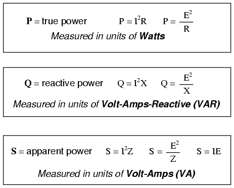
Please note that there are two equations each for the calculation of true and reactive power. There are three equations available for the calculation of apparent power, P=IE being useful only for that purpose. Examine the following circuits and see how these three types of power interrelate for: a purely resistive load in Figurebelow, a purely reactive load in Figure below, and a resistive/reactive load in Figure below.
Resistive Load Only
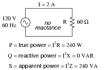
True power, reactive power, and apparent power for a purely resistive load.
Reactive Load Only
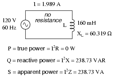
True power, reactive power, and apparent power for a purely reactive load.
Resistive/Reactive Load
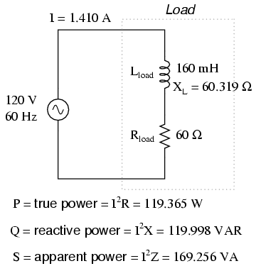
True power, reactive power, and apparent power for a resistive/reactive load.
The Power Triangle
These three types of power—true, reactive, and apparent—relate to one another in trigonometric form. We call this the power triangle: (Figure below).
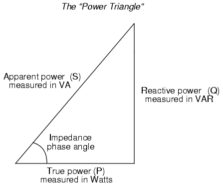
Power triangle relating appearant power to true power and reactive power.
Using the laws of trigonometry, we can solve for the length of any side (amount of any type of power), given the lengths of the other two sides, or the length of one side and an angle.
Review
- Power dissipated by a load is referred to as true power. True power is symbolized by the letter P and is measured in the unit of Watts (W).
- Power merely absorbed and returned in load due to its reactive properties is referred to as reactive power. Reactive power is symbolized by the letter Q and is measured in the unit of Volt-Amps-Reactive (VAR).
- Total power in an AC circuit, both dissipated and absorbed/returned is referred to as apparent power. Apparent power is symbolized by the letter S and is measured in the unit of Volt-Amps (VA).
- These three types of power are trigonometrically related to one another. In a right triangle, P = adjacent length, Q = opposite length, and S = hypotenuse length. The opposite angle is equal to the circuit’s impedance (Z) phase angle.


