10.1: What is Network Analysis?
- Page ID
- 961
\( \newcommand{\vecs}[1]{\overset { \scriptstyle \rightharpoonup} {\mathbf{#1}} } \)
\( \newcommand{\vecd}[1]{\overset{-\!-\!\rightharpoonup}{\vphantom{a}\smash {#1}}} \)
\( \newcommand{\id}{\mathrm{id}}\) \( \newcommand{\Span}{\mathrm{span}}\)
( \newcommand{\kernel}{\mathrm{null}\,}\) \( \newcommand{\range}{\mathrm{range}\,}\)
\( \newcommand{\RealPart}{\mathrm{Re}}\) \( \newcommand{\ImaginaryPart}{\mathrm{Im}}\)
\( \newcommand{\Argument}{\mathrm{Arg}}\) \( \newcommand{\norm}[1]{\| #1 \|}\)
\( \newcommand{\inner}[2]{\langle #1, #2 \rangle}\)
\( \newcommand{\Span}{\mathrm{span}}\)
\( \newcommand{\id}{\mathrm{id}}\)
\( \newcommand{\Span}{\mathrm{span}}\)
\( \newcommand{\kernel}{\mathrm{null}\,}\)
\( \newcommand{\range}{\mathrm{range}\,}\)
\( \newcommand{\RealPart}{\mathrm{Re}}\)
\( \newcommand{\ImaginaryPart}{\mathrm{Im}}\)
\( \newcommand{\Argument}{\mathrm{Arg}}\)
\( \newcommand{\norm}[1]{\| #1 \|}\)
\( \newcommand{\inner}[2]{\langle #1, #2 \rangle}\)
\( \newcommand{\Span}{\mathrm{span}}\) \( \newcommand{\AA}{\unicode[.8,0]{x212B}}\)
\( \newcommand{\vectorA}[1]{\vec{#1}} % arrow\)
\( \newcommand{\vectorAt}[1]{\vec{\text{#1}}} % arrow\)
\( \newcommand{\vectorB}[1]{\overset { \scriptstyle \rightharpoonup} {\mathbf{#1}} } \)
\( \newcommand{\vectorC}[1]{\textbf{#1}} \)
\( \newcommand{\vectorD}[1]{\overrightarrow{#1}} \)
\( \newcommand{\vectorDt}[1]{\overrightarrow{\text{#1}}} \)
\( \newcommand{\vectE}[1]{\overset{-\!-\!\rightharpoonup}{\vphantom{a}\smash{\mathbf {#1}}}} \)
\( \newcommand{\vecs}[1]{\overset { \scriptstyle \rightharpoonup} {\mathbf{#1}} } \)
\( \newcommand{\vecd}[1]{\overset{-\!-\!\rightharpoonup}{\vphantom{a}\smash {#1}}} \)
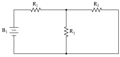
\(\newcommand{\avec}{\mathbf a}\) \(\newcommand{\bvec}{\mathbf b}\) \(\newcommand{\cvec}{\mathbf c}\) \(\newcommand{\dvec}{\mathbf d}\) \(\newcommand{\dtil}{\widetilde{\mathbf d}}\) \(\newcommand{\evec}{\mathbf e}\) \(\newcommand{\fvec}{\mathbf f}\) \(\newcommand{\nvec}{\mathbf n}\) \(\newcommand{\pvec}{\mathbf p}\) \(\newcommand{\qvec}{\mathbf q}\) \(\newcommand{\svec}{\mathbf s}\) \(\newcommand{\tvec}{\mathbf t}\) \(\newcommand{\uvec}{\mathbf u}\) \(\newcommand{\vvec}{\mathbf v}\) \(\newcommand{\wvec}{\mathbf w}\) \(\newcommand{\xvec}{\mathbf x}\) \(\newcommand{\yvec}{\mathbf y}\) \(\newcommand{\zvec}{\mathbf z}\) \(\newcommand{\rvec}{\mathbf r}\) \(\newcommand{\mvec}{\mathbf m}\) \(\newcommand{\zerovec}{\mathbf 0}\) \(\newcommand{\onevec}{\mathbf 1}\) \(\newcommand{\real}{\mathbb R}\) \(\newcommand{\twovec}[2]{\left[\begin{array}{r}#1 \\ #2 \end{array}\right]}\) \(\newcommand{\ctwovec}[2]{\left[\begin{array}{c}#1 \\ #2 \end{array}\right]}\) \(\newcommand{\threevec}[3]{\left[\begin{array}{r}#1 \\ #2 \\ #3 \end{array}\right]}\) \(\newcommand{\cthreevec}[3]{\left[\begin{array}{c}#1 \\ #2 \\ #3 \end{array}\right]}\) \(\newcommand{\fourvec}[4]{\left[\begin{array}{r}#1 \\ #2 \\ #3 \\ #4 \end{array}\right]}\) \(\newcommand{\cfourvec}[4]{\left[\begin{array}{c}#1 \\ #2 \\ #3 \\ #4 \end{array}\right]}\) \(\newcommand{\fivevec}[5]{\left[\begin{array}{r}#1 \\ #2 \\ #3 \\ #4 \\ #5 \\ \end{array}\right]}\) \(\newcommand{\cfivevec}[5]{\left[\begin{array}{c}#1 \\ #2 \\ #3 \\ #4 \\ #5 \\ \end{array}\right]}\) \(\newcommand{\mattwo}[4]{\left[\begin{array}{rr}#1 \amp #2 \\ #3 \amp #4 \\ \end{array}\right]}\) \(\newcommand{\laspan}[1]{\text{Span}\{#1\}}\) \(\newcommand{\bcal}{\cal B}\) \(\newcommand{\ccal}{\cal C}\) \(\newcommand{\scal}{\cal S}\) \(\newcommand{\wcal}{\cal W}\) \(\newcommand{\ecal}{\cal E}\) \(\newcommand{\coords}[2]{\left\{#1\right\}_{#2}}\) \(\newcommand{\gray}[1]{\color{gray}{#1}}\) \(\newcommand{\lgray}[1]{\color{lightgray}{#1}}\) \(\newcommand{\rank}{\operatorname{rank}}\) \(\newcommand{\row}{\text{Row}}\) \(\newcommand{\col}{\text{Col}}\) \(\renewcommand{\row}{\text{Row}}\) \(\newcommand{\nul}{\text{Nul}}\) \(\newcommand{\var}{\text{Var}}\) \(\newcommand{\corr}{\text{corr}}\) \(\newcommand{\len}[1]{\left|#1\right|}\) \(\newcommand{\bbar}{\overline{\bvec}}\) \(\newcommand{\bhat}{\widehat{\bvec}}\) \(\newcommand{\bperp}{\bvec^\perp}\) \(\newcommand{\xhat}{\widehat{\xvec}}\) \(\newcommand{\vhat}{\widehat{\vvec}}\) \(\newcommand{\uhat}{\widehat{\uvec}}\) \(\newcommand{\what}{\widehat{\wvec}}\) \(\newcommand{\Sighat}{\widehat{\Sigma}}\) \(\newcommand{\lt}{<}\) \(\newcommand{\gt}{>}\) \(\newcommand{\amp}{&}\) \(\definecolor{fillinmathshade}{gray}{0.9}\)To illustrate how even a simple circuit can defy analysis by breakdown into series and parallel portions, take start with this series-parallel circuit:

To analyze the above circuit, one would first find the equivalent of R2 and R3 in parallel, then add R1 in series to arrive at a total resistance. Then, taking the voltage of battery B1 with that total circuit resistance, the total current could be calculated through the use of Ohm’s Law (I=E/R), then that current figure used to calculate voltage drops in the circuit. All in all, a fairly simple procedure.
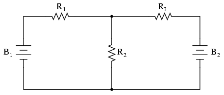
However, the addition of just one more battery could change all of that:

Resistors R2 and R3 are no longer in parallel with each other, because B2 has been inserted into R3‘s branch of the circuit. Upon closer inspection, it appears there are no two resistors in this circuit directly in series or parallel with each other. This is the crux of our problem: in series-parallel analysis, we started off by identifying sets of resistors that were directly in series or parallel with each other, reducing them to single equivalent resistances. If there are no resistors in a simple series or parallel configuration with each other, then what can we do?
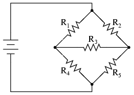
It should be clear that this seemingly simple circuit, with only three resistors, is impossible to reduce as a combination of simple series and simple parallel sections: it is something different altogether. However, this is not the only type of circuit defying series/parallel analysis:

Here we have a bridge circuit, and for the sake of example we will suppose that it is not balanced (ratio R1/R4 not equal to ratio R2/R5). If it were balanced, there would be zero current through R3, and it could be approached as a series/parallel combination circuit (R1—R4 // R2—R5). However, any current through R3makes a series/parallel analysis impossible. R1 is not in series with R4 because there’s another path for electrons to flow through R3. Neither is R2 in series with R5 for the same reason. Likewise, R1 is not in parallel with R2 because R3 is separating their bottom leads. Neither is R4 in parallel with R5. Aaarrggghhhh!
Although it might not be apparent at this point, the heart of the problem is the existence of multiple unknown quantities. At least in a series/parallel combination circuit, there was a way to find total resistance and total voltage, leaving total current as a single unknown value to calculate (and then that current was used to satisfy previously unknown variables in the reduction process until the entire circuit could be analyzed). With these problems, more than one parameter (variable) is unknown at the most basic level of circuit simplification.
With the two-battery circuit, there is no way to arrive at a value for “total resistance,” because there are twosources of power to provide voltage and current (we would need two “total” resistances in order to proceed with any Ohm’s Law calculations). With the unbalanced bridge circuit, there is such a thing as total resistance across the one battery (paving the way for a calculation of total current), but that total current immediately splits up into unknown proportions at each end of the bridge, so no further Ohm’s Law calculations for voltage (E=IR) can be carried out.
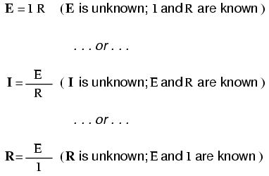
So what can we do when we’re faced with multiple unknowns in a circuit? The answer is initially found in a mathematical process known as simultaneous equations or systems of equations, whereby multiple unknown variables are solved by relating them to each other in multiple equations. In a scenario with only one unknown (such as every Ohm’s Law equation we’ve dealt with thus far), there only needs to be a single equation to solve for the single unknown:

However, when we’re solving for multiple unknown values, we need to have the same number of equations as we have unknowns in order to reach a solution. There are several methods of solving simultaneous equations, all rather intimidating and all too complex for explanation in this chapter. However, many scientific and programmable calculators are able to solve for simultaneous unknowns, so it is recommended to use such a calculator when first learning how to analyze these circuits.
This is not as scary as it may seem at first. Trust me!
Later on we’ll see that some clever people have found tricks to avoid having to use simultaneous equations on these types of circuits. We call these tricks network theorems, and we will explore a few later in this chapter.
Review
- Some circuit configurations (“networks”) cannot be solved by reduction according to series/parallel circuit rules, due to multiple unknown values.
- Mathematical techniques to solve for multiple unknowns (called “simultaneous equations” or “systems”) can be applied to basic Laws of circuits to solve networks.


