11.5: Finite State Machines

Up to now, every circuit that was presented was a combinatorial circuit. That means that its output is dependent only by its current inputs. Previous inputs for that type of circuits have no effect on the output.

However, there are many applications where there is a need for our circuits to have “memory”; to remember previous inputs and calculate their outputs according to them. A circuit whose output depends not only on the present input but also on the history of the input is called a sequential circuit.

In this section we will learn how to design and build such sequential circuits. In order to see how this procedure works, we will use an example, on which we will study our topic.

So let’s suppose we have a digital quiz game that works on a clock and reads an input from a manual button. However, we want the switch to transmit only one HIGH pulse to the circuit. If we hook the button directly on the game circuit it will transmit HIGH for as few clock cycles as our finger can achieve. On a common clock frequency our finger can never be fast enough.

The design procedure has specific steps that must be followed in order to get the work done:

Step 1

The first step of the design procedure is to define with simple but clear words what we want our circuit to do:
“Our mission is to design a secondary circuit that will transmit a HIGH pulse with duration of only one cycle when the manual button is pressed, and won’t transmit another pulse until the button is depressed and pressed again.” Step 2

The next step is to design a State Diagram. This is a diagram that is made from circles and arrows and describes visually the operation of our circuit. In mathematic terms, this diagram that describes the operation of our sequential circuit is a Finite State Machine.

Make a note that this is a Moore Finite State Machine. Its output is a function of only its current state, not its input. That is in contrast with the Mealy Finite State Machine, where input affects the output. In this tutorial, only the Moore Finite State Machine will be examined.

The State Diagram of our circuit is the following: (Figure below)

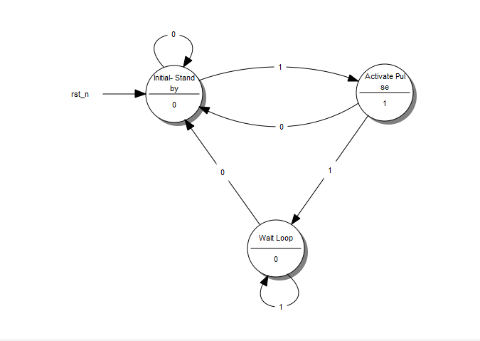
A State Diagram

Every circle represents a “state”, a well-defined condition that our machine can be found at.
In the upper half of the circle we describe that condition. The description helps us remember what our circuit is supposed to do at that condition.

• The first circle is the “stand-by” condition. This is where our circuit starts from and where it waits for another button press.
• The second circle is the condition where the button has just been just pressed and our circuit needs to transmit a HIGH pulse.
• The third circle is the condition where our circuit waits for the button to be released before it returns to the “stand-by” condition.

In the lower part of the circle is the output of our circuit. If we want our circuit to transmit a HIGH on a specific state, we put a 1 on that state. Otherwise we put a 0.

Every arrow represents a “transition” from one state to another. A transition happens once every clock cycle. Depending on the current Input, we may go to a different state each time. Notice the number in the middle of every arrow. This is the current Input.
For example, when we are in the “Initial-Stand by” state and we “read” a 1, the diagram tells us that we have to go to the “Activate Pulse” state. If we read a 0 we must stay on the “Initial-Stand by” state.

So, what does our “Machine” do exactly? It starts from the “Initial - Stand by” state and waits until a 1 is read at the Input. Then it goes to the “Activate Pulse” state and transmits a HIGH pulse on its output. If the button keeps being pressed, the circuit goes to the third state, the “Wait Loop”. There it waits until the button is released (Input goes 0) while transmitting a LOW on the output. Then it’s all over again!

This is possibly the most difficult part of the design procedure, because it cannot be described by simple steps. It takes exprerience and a bit of sharp thinking in order to set up a State Diagram, but the rest is just a set of predetermined steps.

Step 3

Next, we replace the words that describe the different states of the diagram with binary numbers. We start the enumeration from 0 which is assigned on the initial state. We then continue the enumeration with any state we like, until all states have their number. The result looks something like this: (Figure below)

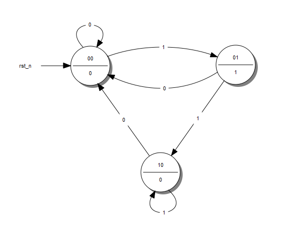
A State Diagram with Coded States

Step 4

Afterwards, we fill the State Table. This table has a very specific form. I will give the table of our example and use it to explain how to fill it in. (Figure below)

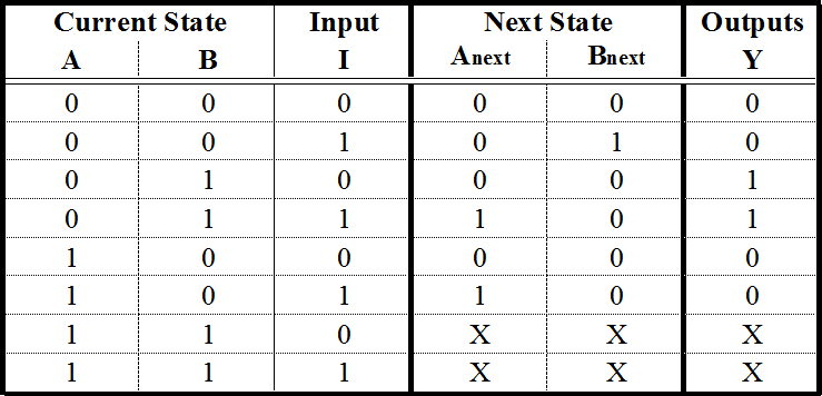
A State Table

The first columns are as many as the bits of the highest number we assigned the State Diagram. If we had 5 states, we would have used up to the number 100, which means we would use 3 columns. For our example, we used up to the number 10, so only 2 columns will be needed. These columns describe the Current Stateof our circuit.
To the right of the Current State columns we write the Input Columns. These will be as many as our Input variables. Our example has only one Input.
Next, we write the Next State Columns. These are as many as the Current State columns.
Finally, we write the Outputs Columns. These are as many as our outputs. Our example has only one output. Since we have built a More Finite State Machine, the output is dependent on only the current input states. This is the reason the outputs column has two 1: to result in an output Boolean function that is independant of input I. Keep on reading for further details.

The Current State and Input columns are the Inputs of our table. We fill them in with all the binary numbers from 0 to

It is simpler than it sounds fortunately. Usually there will be more rows than the actual States we have created in the State Diagram, but that’s ok.

Each row of the Next State columns is filled as follows: We fill it in with the state that we reach when, in the State Diagram, from the Current State of the same row we follow the Input of the same row. If have to fill in a row whose Current State number doesn’t correspond to any actual State in the State Diagram we fill it with Don’t Care terms (X). After all, we don’t care where we can go from a State that doesn’t exist. We wouldn’t be there in the first place! Again it is simpler than it sounds.

The outputs column is filled by the output of the corresponding Current State in the State Diagram.

The State Table is complete! It describes the behaviour of our circuit as fully as the State Diagram does.

Step 5a

The next step is to take that theoretical “Machine” and implement it in a circuit. Most often than not, this implementation involves Flip Flops. This guide is dedicated to this kind of implementation and will describe the procedure for both D - Flip Flops as well as JK - Flip Flops. T - Flip Flops will not be included as they are too similar to the two previous cases. The selection of the Flip Flop to use is arbitrary and usually is determined by cost factors. The best choice is to perform both analysis and decide which type of Flip Flop results in minimum number of logic gates and lesser cost.

First we will examine how we implement our “Machine” with D-Flip Flops.

We will need as many D - Flip Flops as the State columns, 2 in our example. For every Flip Flop we will add one more column in our State table (Figure below) with the name of the Flip Flop’s input, “D” for this case. The column that corresponds to each Flip Flop describes what input we must give the Flip Flop in order to go from the Current State to the Next State. For the D - Flip Flop this is easy: The necessary input is equal to the Next State. In the rows that contain X’s we fill X’s in this column as well.

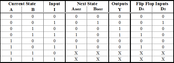
A State Table with D - Flip Flop Excitations

Step 5b

We can do the same steps with JK - Flip Flops. There are some differences however. A JK - Flip Flop has two inputs, therefore we need to add two columns for each Flip Flop. The content of each cell is dictated by the JK’s excitation table:

(Figure below) JK - Flip Flop Excitation Table :

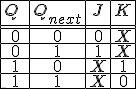
This table says that if we want to go from State Q to State Q_next, we need to use the specific input for each terminal. For example, to go from 0 to 1, we need to feed J with 1 and we don’t care which input we feed to terminal K.

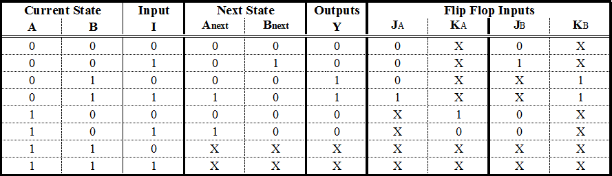
A State Table with JK - Flip Flop Excitations

Step 6

We are in the final stage of our procedure. What remains, is to determine the Boolean functions that produce the inputs of our Flip Flops and the Output. We will extract one Boolean funtion for each Flip Flop input we have. This can be done with a Karnaugh Map. The input variables of this map are the Current State variables as well as the Inputs.

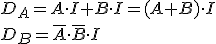
That said, the input functions for our D - Flip Flops are the following: (Figure below)

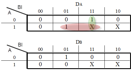
Karnaugh Maps for the D - Flip Flop Inputs

If we chose to use JK - Flip Flops our functions would be the following: (Figure below)

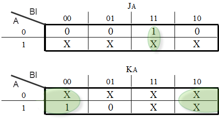
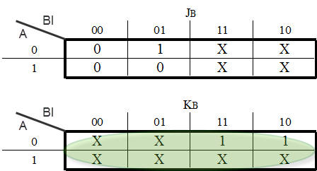
Karnaugh Map for the JK - Flip Flop Input

A Karnaugh Map will be used to determine the function of the Output as well: (Figure below)

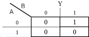
Karnaugh Map for the Output variable Y

Step 7

We design our circuit. We place the Flip Flops and use logic gates to form the Boolean functions that we calculated. The gates take input from the output of the Flip Flops and the Input of the circuit. Don’t forget to connect the clock to the Flip Flops!

The D - Flip Flop version: (Figure below)

The completed D - Flip Flop Sequential Circuit

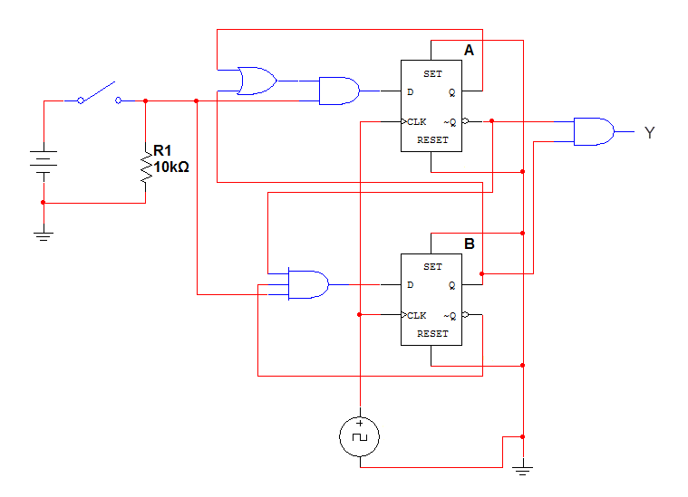
The JK - Flip Flop version: (Figure below)

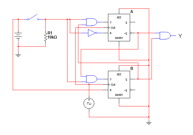
The completed JK - Flip Flop Sequential Circuit

This is it! We have successfully designed and constructed a Sequential Circuit. At first it might seem a daunting task, but after practice and repetition the procedure will become trivial. Sequential Circuits can come in handy as control parts of bigger circuits and can perform any sequential logic task that we can think of. The sky is the limit! (or the circuit board, at least)

Review

• A Sequential Logic function has a “memory” feature and takes into account past inputs in order to decide on the output.
• The Finite State Machine is an abstract mathematical model of a sequential logic function. It has finite inputs, outputs and number of states.
• FSMs are implemented in real-life circuits through the use of Flip Flops
• The implementation procedure needs a specific order of steps (algorithm), in order to be carried out.