
1.2.2.2: Hardware
- Page ID
- 39383
\( \newcommand{\vecs}[1]{\overset { \scriptstyle \rightharpoonup} {\mathbf{#1}} } \)
\( \newcommand{\vecd}[1]{\overset{-\!-\!\rightharpoonup}{\vphantom{a}\smash {#1}}} \)
\( \newcommand{\id}{\mathrm{id}}\) \( \newcommand{\Span}{\mathrm{span}}\)
( \newcommand{\kernel}{\mathrm{null}\,}\) \( \newcommand{\range}{\mathrm{range}\,}\)
\( \newcommand{\RealPart}{\mathrm{Re}}\) \( \newcommand{\ImaginaryPart}{\mathrm{Im}}\)
\( \newcommand{\Argument}{\mathrm{Arg}}\) \( \newcommand{\norm}[1]{\| #1 \|}\)
\( \newcommand{\inner}[2]{\langle #1, #2 \rangle}\)
\( \newcommand{\Span}{\mathrm{span}}\)
\( \newcommand{\id}{\mathrm{id}}\)
\( \newcommand{\Span}{\mathrm{span}}\)
\( \newcommand{\kernel}{\mathrm{null}\,}\)
\( \newcommand{\range}{\mathrm{range}\,}\)
\( \newcommand{\RealPart}{\mathrm{Re}}\)
\( \newcommand{\ImaginaryPart}{\mathrm{Im}}\)
\( \newcommand{\Argument}{\mathrm{Arg}}\)
\( \newcommand{\norm}[1]{\| #1 \|}\)
\( \newcommand{\inner}[2]{\langle #1, #2 \rangle}\)
\( \newcommand{\Span}{\mathrm{span}}\) \( \newcommand{\AA}{\unicode[.8,0]{x212B}}\)
\( \newcommand{\vectorA}[1]{\vec{#1}} % arrow\)
\( \newcommand{\vectorAt}[1]{\vec{\text{#1}}} % arrow\)
\( \newcommand{\vectorB}[1]{\overset { \scriptstyle \rightharpoonup} {\mathbf{#1}} } \)
\( \newcommand{\vectorC}[1]{\textbf{#1}} \)
\( \newcommand{\vectorD}[1]{\overrightarrow{#1}} \)
\( \newcommand{\vectorDt}[1]{\overrightarrow{\text{#1}}} \)
\( \newcommand{\vectE}[1]{\overset{-\!-\!\rightharpoonup}{\vphantom{a}\smash{\mathbf {#1}}}} \)
\( \newcommand{\vecs}[1]{\overset { \scriptstyle \rightharpoonup} {\mathbf{#1}} } \)
\( \newcommand{\vecd}[1]{\overset{-\!-\!\rightharpoonup}{\vphantom{a}\smash {#1}}} \)
\(\newcommand{\avec}{\mathbf a}\) \(\newcommand{\bvec}{\mathbf b}\) \(\newcommand{\cvec}{\mathbf c}\) \(\newcommand{\dvec}{\mathbf d}\) \(\newcommand{\dtil}{\widetilde{\mathbf d}}\) \(\newcommand{\evec}{\mathbf e}\) \(\newcommand{\fvec}{\mathbf f}\) \(\newcommand{\nvec}{\mathbf n}\) \(\newcommand{\pvec}{\mathbf p}\) \(\newcommand{\qvec}{\mathbf q}\) \(\newcommand{\svec}{\mathbf s}\) \(\newcommand{\tvec}{\mathbf t}\) \(\newcommand{\uvec}{\mathbf u}\) \(\newcommand{\vvec}{\mathbf v}\) \(\newcommand{\wvec}{\mathbf w}\) \(\newcommand{\xvec}{\mathbf x}\) \(\newcommand{\yvec}{\mathbf y}\) \(\newcommand{\zvec}{\mathbf z}\) \(\newcommand{\rvec}{\mathbf r}\) \(\newcommand{\mvec}{\mathbf m}\) \(\newcommand{\zerovec}{\mathbf 0}\) \(\newcommand{\onevec}{\mathbf 1}\) \(\newcommand{\real}{\mathbb R}\) \(\newcommand{\twovec}[2]{\left[\begin{array}{r}#1 \\ #2 \end{array}\right]}\) \(\newcommand{\ctwovec}[2]{\left[\begin{array}{c}#1 \\ #2 \end{array}\right]}\) \(\newcommand{\threevec}[3]{\left[\begin{array}{r}#1 \\ #2 \\ #3 \end{array}\right]}\) \(\newcommand{\cthreevec}[3]{\left[\begin{array}{c}#1 \\ #2 \\ #3 \end{array}\right]}\) \(\newcommand{\fourvec}[4]{\left[\begin{array}{r}#1 \\ #2 \\ #3 \\ #4 \end{array}\right]}\) \(\newcommand{\cfourvec}[4]{\left[\begin{array}{c}#1 \\ #2 \\ #3 \\ #4 \end{array}\right]}\) \(\newcommand{\fivevec}[5]{\left[\begin{array}{r}#1 \\ #2 \\ #3 \\ #4 \\ #5 \\ \end{array}\right]}\) \(\newcommand{\cfivevec}[5]{\left[\begin{array}{c}#1 \\ #2 \\ #3 \\ #4 \\ #5 \\ \end{array}\right]}\) \(\newcommand{\mattwo}[4]{\left[\begin{array}{rr}#1 \amp #2 \\ #3 \amp #4 \\ \end{array}\right]}\) \(\newcommand{\laspan}[1]{\text{Span}\{#1\}}\) \(\newcommand{\bcal}{\cal B}\) \(\newcommand{\ccal}{\cal C}\) \(\newcommand{\scal}{\cal S}\) \(\newcommand{\wcal}{\cal W}\) \(\newcommand{\ecal}{\cal E}\) \(\newcommand{\coords}[2]{\left\{#1\right\}_{#2}}\) \(\newcommand{\gray}[1]{\color{gray}{#1}}\) \(\newcommand{\lgray}[1]{\color{lightgray}{#1}}\) \(\newcommand{\rank}{\operatorname{rank}}\) \(\newcommand{\row}{\text{Row}}\) \(\newcommand{\col}{\text{Col}}\) \(\renewcommand{\row}{\text{Row}}\) \(\newcommand{\nul}{\text{Nul}}\) \(\newcommand{\var}{\text{Var}}\) \(\newcommand{\corr}{\text{corr}}\) \(\newcommand{\len}[1]{\left|#1\right|}\) \(\newcommand{\bbar}{\overline{\bvec}}\) \(\newcommand{\bhat}{\widehat{\bvec}}\) \(\newcommand{\bperp}{\bvec^\perp}\) \(\newcommand{\xhat}{\widehat{\xvec}}\) \(\newcommand{\vhat}{\widehat{\vvec}}\) \(\newcommand{\uhat}{\widehat{\uvec}}\) \(\newcommand{\what}{\widehat{\wvec}}\) \(\newcommand{\Sighat}{\widehat{\Sigma}}\) \(\newcommand{\lt}{<}\) \(\newcommand{\gt}{>}\) \(\newcommand{\amp}{&}\) \(\definecolor{fillinmathshade}{gray}{0.9}\)Introduction
As we start exploring the nuts and bolts of computer hardware, let’s first take a moment to connect it to something you might not immediately think about—agriculture. You might be wondering, "What do computers have to do with agriculture?" Well, a lot more than you might expect!
Picture a modern farm. It’s not just fields and tractors anymore; it’s a high-tech operation where computers are as crucial as any traditional tool. From sensors that monitor soil moisture to drones that survey crops from the sky, computer technology is transforming agriculture into a cutting-edge industry. These advancements aren’t just about making farming easier—they’re about making it smarter, more efficient, and more sustainable.
In this section, we’re going to dive into the world of computer hardware. Understanding these components will not only give you insights into how your personal computer works but also how these technologies are being used to revolutionize agriculture. Whether it’s a CPU crunching numbers to predict the best planting times or sensors feeding data into a system to optimize water usage, the hardware we’ll discuss is the backbone of this agricultural tech revolution.
So, as we get into the details of motherboards, CPUs, and input devices, keep in mind that this isn’t just abstract knowledge—it’s the foundation of the technology that’s feeding the world and pushing the boundaries of what’s possible in farming. Ready to dig in? Let’s get started!
Hardware
Let’s consider the hardware of an information system through an agricultural lens, comparing the various types of computing devices to different agricultural tools and machinery. Hardware is the most visible part of any information system: the equipment such as computers, scanners and printers that is used to capture data, transform it and present it to the user as output. Although we will focus mainly on the personal computer (PC) and the peripheral devices that are commonly used with it, the same principles apply to the complete range of computers:
1. Supercomputers: Think of supercomputers as the heavy-duty tractors or combine harvesters of the tech world. Just as these machines handle the most demanding farming tasks—such as plowing large fields or harvesting massive crops—supercomputers tackle exceptionally complex scientific computations and data processing.
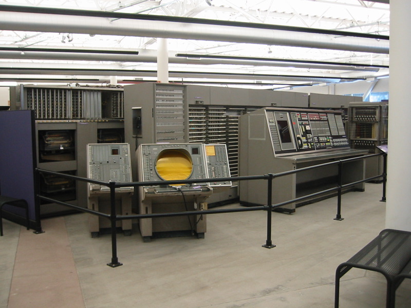
2. Mainframe Computers: These are akin to large-scale irrigation systems or silos that manage and store vast amounts of resources for numerous farms. Mainframes offer substantial processing power and data storage, supporting many users in managing extensive agricultural operations and resources efficiently.
3. Servers: Imagine servers as central grain elevators or cooperative storage facilities. They provide significant storage capacity and enable multiple users (farmers, agronomists, etc.) to access and share resources, although the actual processing—like analyzing crop data—often happens at individual farms (or users' machines).
4. Workstations: Workstations are similar to specialized farm equipment, like high-performance soil testers or precision planters. They offer advanced capabilities for detailed and demanding tasks—such as analyzing soil samples or optimizing planting patterns—allowing farmers to handle complex agricultural computations on their own.
5. Personal Computers: These are like versatile multipurpose farm tools or small tractors. They come with all the basic equipment needed for various tasks (monitor, keyboard, CPU) and can be used independently or as part of a larger system (like a farm management network). They’re flexible and handy for everyday agricultural tasks, such as tracking farm inventories or analyzing crop data.
6. Mobile Devices: Think of mobile devices as portable farming tools—like handheld soil moisture meters or GPS devices. They offer maximum portability and can connect wirelessly to farm management systems, though they don’t replace the full functionality of larger equipment or systems.
7. Wearable Computers: Wearables are akin to advanced monitoring systems for livestock or crops, like automated collars for tracking animal health or sensors embedded in fields to monitor environmental conditions. They provide specialized, real-time data collection for specific agricultural needs.
8. Embedded Computers: These can be compared to integrated systems in modern farm machinery or smart irrigation controllers. They’re built into various appliances (from tractors to weather stations) to handle specific tasks, improving efficiency and functionality within the broader agricultural system.
9. Smart Cards: Finally, smart cards are like digital farm passports or key fobs that provide secure access and identification. They can hold crucial information, such as farm management details, livestock records, or access rights to equipment, streamlining various aspects of farm operations.
By viewing computing hardware through an agricultural lens, we can better understand how each component plays a role in managing, processing, and optimizing agricultural tasks and resources.
- Discovering Information Systems Chapter 4: Hardware. Authored by: Jean-Paul Van Belle, Mike Eccles, and Jane Nash. Located at: https://archive.org/details/ost-computer-science-discoveringinformationsystems. License: CC BY-NC-ND: Attribution-NonCommercial-NoDerivatives
- Mainframe computer. Authored by: Naotake Murayama. Located at: https://www.flickr.com/photos/naotakem/120643390/. License: CC BY: Attribution
- CPU wafer stack. Authored by: Mark Sze. Located at: https://www.flickr.com/photos/marksze/4231114748/. License: CC BY-NC-ND: Attribution-NonCommercial-NoDerivatives
- Computer mouse. Authored by: Geralt. Located at: https://pixabay.com/en/mouse-computer-hardware-input-160032/. License: CC0: No Rights Reserved
- Touch screen devices. Authored by: Geralt. Located at: https://pixabay.com/en/mobile-phone-smartphone-tablet-630412/. License: CC0: No Rights Reserved
- Bar code scanner. Authored by: OpenClipartVectors. Located at: https://pixabay.com/en/bar-code-scanner-bar-code-laser-155766/. License: CC0: No Rights Reserved
- Floppy Disks. Authored by: PublicDomainPictures. Located at: https://pixabay.com/en/floppy-disk-data-computer-214975/. License: CC0: No Rights Reserved
- Inkjet printer. Authored by: OpenClipartVectors. Located at: https://pixabay.com/en/printer-computer-hardware-inkjet-159612/. License: CC0: No Rights Reserved
- VHS tapes. Authored by: wongpear. Located at: https://pixabay.com/en/vhs-video-tapes-recording-398740/. License: CC0: No Rights Reserved
- RAM. Authored by: lrcfree. Located at: https://pixabay.com/en/ram-technology-pc-computer-683250/. License: CC0: No Rights Reserved