1.2.3.1: Reading- Booting
- Page ID
- 37929
\( \newcommand{\vecs}[1]{\overset { \scriptstyle \rightharpoonup} {\mathbf{#1}} } \)
\( \newcommand{\vecd}[1]{\overset{-\!-\!\rightharpoonup}{\vphantom{a}\smash {#1}}} \)
\( \newcommand{\dsum}{\displaystyle\sum\limits} \)
\( \newcommand{\dint}{\displaystyle\int\limits} \)
\( \newcommand{\dlim}{\displaystyle\lim\limits} \)
\( \newcommand{\id}{\mathrm{id}}\) \( \newcommand{\Span}{\mathrm{span}}\)
( \newcommand{\kernel}{\mathrm{null}\,}\) \( \newcommand{\range}{\mathrm{range}\,}\)
\( \newcommand{\RealPart}{\mathrm{Re}}\) \( \newcommand{\ImaginaryPart}{\mathrm{Im}}\)
\( \newcommand{\Argument}{\mathrm{Arg}}\) \( \newcommand{\norm}[1]{\| #1 \|}\)
\( \newcommand{\inner}[2]{\langle #1, #2 \rangle}\)
\( \newcommand{\Span}{\mathrm{span}}\)
\( \newcommand{\id}{\mathrm{id}}\)
\( \newcommand{\Span}{\mathrm{span}}\)
\( \newcommand{\kernel}{\mathrm{null}\,}\)
\( \newcommand{\range}{\mathrm{range}\,}\)
\( \newcommand{\RealPart}{\mathrm{Re}}\)
\( \newcommand{\ImaginaryPart}{\mathrm{Im}}\)
\( \newcommand{\Argument}{\mathrm{Arg}}\)
\( \newcommand{\norm}[1]{\| #1 \|}\)
\( \newcommand{\inner}[2]{\langle #1, #2 \rangle}\)
\( \newcommand{\Span}{\mathrm{span}}\) \( \newcommand{\AA}{\unicode[.8,0]{x212B}}\)
\( \newcommand{\vectorA}[1]{\vec{#1}} % arrow\)
\( \newcommand{\vectorAt}[1]{\vec{\text{#1}}} % arrow\)
\( \newcommand{\vectorB}[1]{\overset { \scriptstyle \rightharpoonup} {\mathbf{#1}} } \)
\( \newcommand{\vectorC}[1]{\textbf{#1}} \)
\( \newcommand{\vectorD}[1]{\overrightarrow{#1}} \)
\( \newcommand{\vectorDt}[1]{\overrightarrow{\text{#1}}} \)
\( \newcommand{\vectE}[1]{\overset{-\!-\!\rightharpoonup}{\vphantom{a}\smash{\mathbf {#1}}}} \)
\( \newcommand{\vecs}[1]{\overset { \scriptstyle \rightharpoonup} {\mathbf{#1}} } \)
\( \newcommand{\vecd}[1]{\overset{-\!-\!\rightharpoonup}{\vphantom{a}\smash {#1}}} \)
\(\newcommand{\avec}{\mathbf a}\) \(\newcommand{\bvec}{\mathbf b}\) \(\newcommand{\cvec}{\mathbf c}\) \(\newcommand{\dvec}{\mathbf d}\) \(\newcommand{\dtil}{\widetilde{\mathbf d}}\) \(\newcommand{\evec}{\mathbf e}\) \(\newcommand{\fvec}{\mathbf f}\) \(\newcommand{\nvec}{\mathbf n}\) \(\newcommand{\pvec}{\mathbf p}\) \(\newcommand{\qvec}{\mathbf q}\) \(\newcommand{\svec}{\mathbf s}\) \(\newcommand{\tvec}{\mathbf t}\) \(\newcommand{\uvec}{\mathbf u}\) \(\newcommand{\vvec}{\mathbf v}\) \(\newcommand{\wvec}{\mathbf w}\) \(\newcommand{\xvec}{\mathbf x}\) \(\newcommand{\yvec}{\mathbf y}\) \(\newcommand{\zvec}{\mathbf z}\) \(\newcommand{\rvec}{\mathbf r}\) \(\newcommand{\mvec}{\mathbf m}\) \(\newcommand{\zerovec}{\mathbf 0}\) \(\newcommand{\onevec}{\mathbf 1}\) \(\newcommand{\real}{\mathbb R}\) \(\newcommand{\twovec}[2]{\left[\begin{array}{r}#1 \\ #2 \end{array}\right]}\) \(\newcommand{\ctwovec}[2]{\left[\begin{array}{c}#1 \\ #2 \end{array}\right]}\) \(\newcommand{\threevec}[3]{\left[\begin{array}{r}#1 \\ #2 \\ #3 \end{array}\right]}\) \(\newcommand{\cthreevec}[3]{\left[\begin{array}{c}#1 \\ #2 \\ #3 \end{array}\right]}\) \(\newcommand{\fourvec}[4]{\left[\begin{array}{r}#1 \\ #2 \\ #3 \\ #4 \end{array}\right]}\) \(\newcommand{\cfourvec}[4]{\left[\begin{array}{c}#1 \\ #2 \\ #3 \\ #4 \end{array}\right]}\) \(\newcommand{\fivevec}[5]{\left[\begin{array}{r}#1 \\ #2 \\ #3 \\ #4 \\ #5 \\ \end{array}\right]}\) \(\newcommand{\cfivevec}[5]{\left[\begin{array}{c}#1 \\ #2 \\ #3 \\ #4 \\ #5 \\ \end{array}\right]}\) \(\newcommand{\mattwo}[4]{\left[\begin{array}{rr}#1 \amp #2 \\ #3 \amp #4 \\ \end{array}\right]}\) \(\newcommand{\laspan}[1]{\text{Span}\{#1\}}\) \(\newcommand{\bcal}{\cal B}\) \(\newcommand{\ccal}{\cal C}\) \(\newcommand{\scal}{\cal S}\) \(\newcommand{\wcal}{\cal W}\) \(\newcommand{\ecal}{\cal E}\) \(\newcommand{\coords}[2]{\left\{#1\right\}_{#2}}\) \(\newcommand{\gray}[1]{\color{gray}{#1}}\) \(\newcommand{\lgray}[1]{\color{lightgray}{#1}}\) \(\newcommand{\rank}{\operatorname{rank}}\) \(\newcommand{\row}{\text{Row}}\) \(\newcommand{\col}{\text{Col}}\) \(\renewcommand{\row}{\text{Row}}\) \(\newcommand{\nul}{\text{Nul}}\) \(\newcommand{\var}{\text{Var}}\) \(\newcommand{\corr}{\text{corr}}\) \(\newcommand{\len}[1]{\left|#1\right|}\) \(\newcommand{\bbar}{\overline{\bvec}}\) \(\newcommand{\bhat}{\widehat{\bvec}}\) \(\newcommand{\bperp}{\bvec^\perp}\) \(\newcommand{\xhat}{\widehat{\xvec}}\) \(\newcommand{\vhat}{\widehat{\vvec}}\) \(\newcommand{\uhat}{\widehat{\uvec}}\) \(\newcommand{\what}{\widehat{\wvec}}\) \(\newcommand{\Sighat}{\widehat{\Sigma}}\) \(\newcommand{\lt}{<}\) \(\newcommand{\gt}{>}\) \(\newcommand{\amp}{&}\) \(\definecolor{fillinmathshade}{gray}{0.9}\)Introduction
Before we dive into the intricacies of booting, let's consider why this process is crucial, especially in the context of agriculture. Booting is the initial process that brings a computerized system to life, allowing it to perform all the tasks it's designed for. In modern agriculture, particularly in regions like California's Central Valley, the efficiency and reliability of this process can make a significant difference in daily operations.
Imagine a farm in the Central Valley that relies on automated irrigation systems, weather monitoring tools, and data analytics to optimize crop yields. Each morning, these systems must boot up and be ready to gather data, analyze conditions, and control machinery. A delay or failure in the booting process could mean missed opportunities to water crops at the optimal time, potentially impacting the entire day's operations. For example, if a system that controls irrigation fails to boot properly, it might not deliver the precise amount of water needed, leading to either overwatering or under-watering, both of which can affect crop health and yield.
Understanding the booting process is not just about knowing how computers start; it's about ensuring that the technology you depend on—whether it’s for running a business or managing a farm—operates smoothly from the moment you power it on. In the context of agriculture, this knowledge is crucial for maintaining the reliability of the systems that are essential to modern farming practices. So, let's get into the details of how booting works and why it’s a foundational aspect of any computerized system.

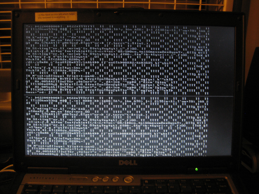
In computing, booting (or booting up) is the initialization of a computerized system. The system can be a computer or a computer appliance. The booting process can be “hard”, after electrical power to the CPU is switched from off to on (in order to diagnose particular hardware errors), or “soft”, when thosepower-on self-tests (POST) can be avoided. Soft booting can be initiated by hardware such as a button press, or by software command. Booting is complete when the normal, operative, runtime environment is attained.
A boot loader is a computer program that loads an operating system or some other system software for the computer after completion of the power-on self-tests; it is the loader for the operating system itself, which has its own loader for loading ordinary user programs and libraries. Within the hard reboot process, it runs after completion of the self-tests, then loads and runs the software. A boot loader is loaded into main memory from persistent memory, such as a hard disk drive or, in some older computers, from a medium such as punched cards, punched tape, or magnetic tape. The boot loader then loads and executes the processes that finalize the boot. Like POST processes, the boot loader code comes from a “hard-wired” and persistent location; if that location is too limited for some reason, that primary boot loader calls a second-stage boot loader or a secondary program loader.
On modern general purpose computers, the boot up process can take tens of seconds, and typically involves performing a power-on self-test, locating and initializing peripheral devices, and then finding, loading and starting an operating system. The process of hibernating or sleeping does not involve booting. Minimally, some embedded systems do not require a noticeable boot sequence to begin functioning and when turned on may simply run operational programs that are stored in ROM. All computing systems are state machines, and a reboot may be the only method to return to a designated zero-state from an unintended, locked state.
Boot is short for bootstrap or bootstrap load and derives from the phrase to pull oneself up by one’s bootstraps. The usage calls attention to the requirement that, if most software is loaded onto a computer by other software already running on the computer, some mechanism must exist to load the initial software onto the computer. Early computers used a variety of ad-hoc methods to get a small program into memory to solve this problem. The invention ofread-only memory (ROM) of various types solved this paradox by allowing computers to be shipped with a start up program that could not be erased. Growth in the capacity of ROM has allowed ever more elaborate start up procedures to be implemented.
- Booting. Provided by: Wikipedia. Located at: https://en.Wikipedia.org/wiki/Booting. License: CC BY-SA: Attribution-ShareAlike
- Booting up. Authored by: Nick Johnson. Located at: https://www.flickr.com/photos/npj/4836485286/. License: CC BY: Attribution

