
4.6: Intro- Interface
- Page ID
- 14765
\( \newcommand{\vecs}[1]{\overset { \scriptstyle \rightharpoonup} {\mathbf{#1}} } \)
\( \newcommand{\vecd}[1]{\overset{-\!-\!\rightharpoonup}{\vphantom{a}\smash {#1}}} \)
\( \newcommand{\dsum}{\displaystyle\sum\limits} \)
\( \newcommand{\dint}{\displaystyle\int\limits} \)
\( \newcommand{\dlim}{\displaystyle\lim\limits} \)
\( \newcommand{\id}{\mathrm{id}}\) \( \newcommand{\Span}{\mathrm{span}}\)
( \newcommand{\kernel}{\mathrm{null}\,}\) \( \newcommand{\range}{\mathrm{range}\,}\)
\( \newcommand{\RealPart}{\mathrm{Re}}\) \( \newcommand{\ImaginaryPart}{\mathrm{Im}}\)
\( \newcommand{\Argument}{\mathrm{Arg}}\) \( \newcommand{\norm}[1]{\| #1 \|}\)
\( \newcommand{\inner}[2]{\langle #1, #2 \rangle}\)
\( \newcommand{\Span}{\mathrm{span}}\)
\( \newcommand{\id}{\mathrm{id}}\)
\( \newcommand{\Span}{\mathrm{span}}\)
\( \newcommand{\kernel}{\mathrm{null}\,}\)
\( \newcommand{\range}{\mathrm{range}\,}\)
\( \newcommand{\RealPart}{\mathrm{Re}}\)
\( \newcommand{\ImaginaryPart}{\mathrm{Im}}\)
\( \newcommand{\Argument}{\mathrm{Arg}}\)
\( \newcommand{\norm}[1]{\| #1 \|}\)
\( \newcommand{\inner}[2]{\langle #1, #2 \rangle}\)
\( \newcommand{\Span}{\mathrm{span}}\) \( \newcommand{\AA}{\unicode[.8,0]{x212B}}\)
\( \newcommand{\vectorA}[1]{\vec{#1}} % arrow\)
\( \newcommand{\vectorAt}[1]{\vec{\text{#1}}} % arrow\)
\( \newcommand{\vectorB}[1]{\overset { \scriptstyle \rightharpoonup} {\mathbf{#1}} } \)
\( \newcommand{\vectorC}[1]{\textbf{#1}} \)
\( \newcommand{\vectorD}[1]{\overrightarrow{#1}} \)
\( \newcommand{\vectorDt}[1]{\overrightarrow{\text{#1}}} \)
\( \newcommand{\vectE}[1]{\overset{-\!-\!\rightharpoonup}{\vphantom{a}\smash{\mathbf {#1}}}} \)
\( \newcommand{\vecs}[1]{\overset { \scriptstyle \rightharpoonup} {\mathbf{#1}} } \)
\(\newcommand{\longvect}{\overrightarrow}\)
\( \newcommand{\vecd}[1]{\overset{-\!-\!\rightharpoonup}{\vphantom{a}\smash {#1}}} \)
\(\newcommand{\avec}{\mathbf a}\) \(\newcommand{\bvec}{\mathbf b}\) \(\newcommand{\cvec}{\mathbf c}\) \(\newcommand{\dvec}{\mathbf d}\) \(\newcommand{\dtil}{\widetilde{\mathbf d}}\) \(\newcommand{\evec}{\mathbf e}\) \(\newcommand{\fvec}{\mathbf f}\) \(\newcommand{\nvec}{\mathbf n}\) \(\newcommand{\pvec}{\mathbf p}\) \(\newcommand{\qvec}{\mathbf q}\) \(\newcommand{\svec}{\mathbf s}\) \(\newcommand{\tvec}{\mathbf t}\) \(\newcommand{\uvec}{\mathbf u}\) \(\newcommand{\vvec}{\mathbf v}\) \(\newcommand{\wvec}{\mathbf w}\) \(\newcommand{\xvec}{\mathbf x}\) \(\newcommand{\yvec}{\mathbf y}\) \(\newcommand{\zvec}{\mathbf z}\) \(\newcommand{\rvec}{\mathbf r}\) \(\newcommand{\mvec}{\mathbf m}\) \(\newcommand{\zerovec}{\mathbf 0}\) \(\newcommand{\onevec}{\mathbf 1}\) \(\newcommand{\real}{\mathbb R}\) \(\newcommand{\twovec}[2]{\left[\begin{array}{r}#1 \\ #2 \end{array}\right]}\) \(\newcommand{\ctwovec}[2]{\left[\begin{array}{c}#1 \\ #2 \end{array}\right]}\) \(\newcommand{\threevec}[3]{\left[\begin{array}{r}#1 \\ #2 \\ #3 \end{array}\right]}\) \(\newcommand{\cthreevec}[3]{\left[\begin{array}{c}#1 \\ #2 \\ #3 \end{array}\right]}\) \(\newcommand{\fourvec}[4]{\left[\begin{array}{r}#1 \\ #2 \\ #3 \\ #4 \end{array}\right]}\) \(\newcommand{\cfourvec}[4]{\left[\begin{array}{c}#1 \\ #2 \\ #3 \\ #4 \end{array}\right]}\) \(\newcommand{\fivevec}[5]{\left[\begin{array}{r}#1 \\ #2 \\ #3 \\ #4 \\ #5 \\ \end{array}\right]}\) \(\newcommand{\cfivevec}[5]{\left[\begin{array}{c}#1 \\ #2 \\ #3 \\ #4 \\ #5 \\ \end{array}\right]}\) \(\newcommand{\mattwo}[4]{\left[\begin{array}{rr}#1 \amp #2 \\ #3 \amp #4 \\ \end{array}\right]}\) \(\newcommand{\laspan}[1]{\text{Span}\{#1\}}\) \(\newcommand{\bcal}{\cal B}\) \(\newcommand{\ccal}{\cal C}\) \(\newcommand{\scal}{\cal S}\) \(\newcommand{\wcal}{\cal W}\) \(\newcommand{\ecal}{\cal E}\) \(\newcommand{\coords}[2]{\left\{#1\right\}_{#2}}\) \(\newcommand{\gray}[1]{\color{gray}{#1}}\) \(\newcommand{\lgray}[1]{\color{lightgray}{#1}}\) \(\newcommand{\rank}{\operatorname{rank}}\) \(\newcommand{\row}{\text{Row}}\) \(\newcommand{\col}{\text{Col}}\) \(\renewcommand{\row}{\text{Row}}\) \(\newcommand{\nul}{\text{Nul}}\) \(\newcommand{\var}{\text{Var}}\) \(\newcommand{\corr}{\text{corr}}\) \(\newcommand{\len}[1]{\left|#1\right|}\) \(\newcommand{\bbar}{\overline{\bvec}}\) \(\newcommand{\bhat}{\widehat{\bvec}}\) \(\newcommand{\bperp}{\bvec^\perp}\) \(\newcommand{\xhat}{\widehat{\xvec}}\) \(\newcommand{\vhat}{\widehat{\vvec}}\) \(\newcommand{\uhat}{\widehat{\uvec}}\) \(\newcommand{\what}{\widehat{\wvec}}\) \(\newcommand{\Sighat}{\widehat{\Sigma}}\) \(\newcommand{\lt}{<}\) \(\newcommand{\gt}{>}\) \(\newcommand{\amp}{&}\) \(\definecolor{fillinmathshade}{gray}{0.9}\)https://www.jegsworks.com/lessons/numbers-2/intro/interface.htm
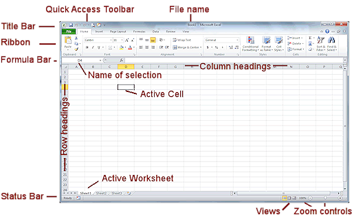
If you have worked with Windows programs before, you already know a lot about Excel's window. It has all the normal window parts, like the Status bar, Title bar, scroll bars. The Excel window is actually a lot like what you saw in Word. If you are not familiar with Word, you should consider working at least the first project of Working with Words: Word 2007, 2010, 2013, and 2016 before continuing. The lessons in Working with Numbers assume that you are somewhat experienced with basic word processing skills.
Spreadsheet Terms
| Term | Explanation |
|---|---|
| spreadsheet | Document that is entirely made up of rows and columns. Used to list and analyze data.
|
| workbook | The basic document for Excel. The default workbook name is Book1.xlsx where the extension xlsx seems to come from 'Excel spreadsheet in XML format'. Older versions of Excel use a different format, xls. |
| worksheet |
A single sheet of data. One or more worksheets make a workbook.
Think of them as pieces of paper that are stacked on top of each other to form the workbook. The default workbook contains three worksheets, named Sheet1, Sheet2, Sheet3. (Excel 2016 has only 1 sheet by default) You will want to change these names to something more interesting and helpful! The maximum number of worksheets in a workbook depends on your computer's memory. A worksheet, also called just a sheet or spreadsheet, can have up to 1,048,576 rows by 16,384 columns with up to 32,767 characters in a single cell. This is enough for most purposes! |
| workbook window | The document window inside an Excel window. (See next section for illustrations) |
| columns | Named with letters in the following pattern: A, B, C,…Z, AA, AB, AC,…AZ, BA, BB, BC,…BZ, CA,…IA, IB,…IV... XFD, which is the last column possible. |
| rows | Named with numbers from 1 to 1,048,576. |
| cell | Intersection of a row and a column on a worksheet. |
| active cell | 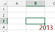  Has a dark border around it and the row and column headers are colored. Has a dark border around it and the row and column headers are colored.This is the cell that receives your keystrokes and commands. You make a cell the active cell when you select it, by clicking it or by moving into it with keys. The TAB or the arrow keys are handy for moving from cell to cell. |
| grid lines |  The gray lines that form the cells. By default they don't print. The gray lines that form the cells. By default they don't print.
If you want to print the gridlines, there is a check box in the Page Setup dialog |
| sheet tab |
|
| active worksheet | The worksheet that receives your keystrokes and commands. It has a white sheet tab with its name in bold. If you group two or more worksheets together, you can have more than one active sheet. This is a cool feature, when it is not a disaster because you did not realize that your typing was going to show up on more than one sheet! |
| workspace | The area below the ribbon that holds your documents |

 Each worksheet has a tab at the bottom of the workbook window with the name of the worksheet on it.
 Excel 2007, 2010: Multiple Windows Inside Excel Window

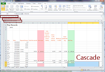
An Excel 2007 or 2010 window can contain several open workbooks at the same time. This Multiple Document Interface is the way older Office programs worked. (Excel 2013 and 2016 put each document in its own complete window like other Office 2013 and 2016 programs.)
By default each document is maximized inside the master Excel window, like the illustration above. You cannot tell from looking at the Excel window how many documents are open.
How to tell how many documents are open:
- Switch Windows button: On the View tab click the Switch Windows button to get a list of all open Excel documents.
- Taskbar: Depending on your version of Windows, the Windows Taskbar shows multiple Excel icons or a single icon with a right click menu listing the open documents.
To show a document in a separate window:
Open a new instance of Excel and then open the file that you want to see in it from inside Excel.
Arranging documents inside the Excel window:
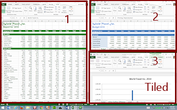
You can show more than one workbook window at a time inside the big Excel window by lining them up in different ways. The illustration above shows two cascading windows inside the master Excel window. The windows have been resized from the default sizes. The master window has the ribbon.
To arrange document windows inside the Excel window, you can open the Arrange Windows dialog, View tab > Arrange All button. A dialog opens where you can choose an arrangement. Notice that there are a number of choices in this tab group!


You can also drag the document window edges to resize each one. Each document has its own Minimize, Maximize, and Close buttons. Minimizing a window minimizes it to the bottom of the Excel window, not to the Taskbar.

 Excel 2013, 2016: Separate Windows
Excel 2013 and 2016 put each workbook into its own window with its own ribbon. It no longer allows multiple workbooks to show inside one main window. Excel has finally caught up with other Office programs with this behavior.
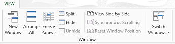
The View ribbon tab has buttons to help you manage your Excel windows.
The New Window button lets you open your current spreadsheet in a new window where you can pick a different sheet tab or show a different section of the current sheet. You still have just one document with Excel synchronizing the changes you make.
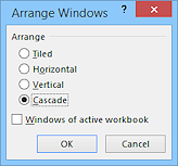
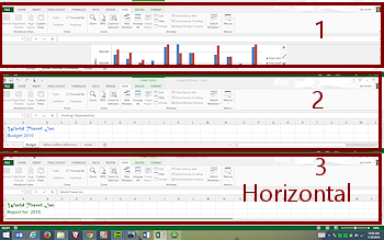
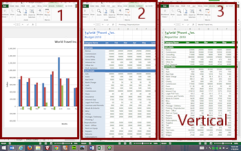
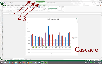
The Arrange All button opens a dialog that lets you pick how you want to arrange the open Excel windows on the screen - Tiled, Horizontal, Vertical, or Cascade.
![]() Active Worksheets Only: The check box 'Windows of active workbook' restricts the arranging to windows that show part of the current workbook. Uncheck that box to arrange windows containing different workbooks.
Active Worksheets Only: The check box 'Windows of active workbook' restricts the arranging to windows that show part of the current workbook. Uncheck that box to arrange windows containing different workbooks.
The Worksheet & Formula Bar
The Formula Bar is a feature that is special to a spreadsheet program. To help keep life confusing, the term Formula Bar is used both for the whole bar you see above the cells and also for just the text box on the right above the cells, which displays what is in the selected cell. In older versions of Excel, you had to do all editing in the Formula Bar but recent versions let you edit directly in the cell. Much better!
The Formula bar behaves the same in Excel 2007, 2010, 2013, and 2016, except from some color differences.
The Name Box shows the cell reference for the current cell or for the upper left cell of the current selection or the name of the selected cell or range of cells.
The buttons to the right of the Name Box apply to the Formula Bar.
 Cancel: Clears any changes.
 Enter: Accepts changes and exits Edit mode. More typing will replace cell contents.
 Insert Formula: Opens a dialog where you can choose one of Excel's pre-defined formulas. That dialog then opens the Function Arguments dialog, which has text boxes for you to fill in. No risk of typing errors messing up the formula you meant to enter!
Worksheet Terms
| Term | Explanation |
|---|---|
| headings | The buttons at the top of columns (letters) and at the left end of rows (numbers). For a selected column or row the heading is colored. |
| enter data | Select the cell, type your data, and press the ENTER key or click the Enter button |
| Name Box | At the top left above the sheet cells and headings. Used to display cell references and to assign and display names for a cell or a range of cells. |
| range |  A rectangular set of cells, referred to by using the upper left and lower right cell references with a colon between them, like A2:C5 for the range illustrated at the right. The absolute reference for the range would be $A$2:$C$5. A rectangular set of cells, referred to by using the upper left and lower right cell references with a colon between them, like A2:C5 for the range illustrated at the right. The absolute reference for the range would be $A$2:$C$5.You select a range by dragging, for example from the upper left cell to the lower right cell. As you drag, the Name Box shows the number of rows and columns that are selected. Once you quit dragging, the Name Box displays the upper left cell only. |
| Formula bar |  Shows the contents of a selected cell, whether it is plain text, numbers, or a formula. Sometimes the whole bar that contains the Name Box and the formula text box is called the Formula bar. Sometimes just the text box that shows the formula or text is meant. Shows the contents of a selected cell, whether it is plain text, numbers, or a formula. Sometimes the whole bar that contains the Name Box and the formula text box is called the Formula bar. Sometimes just the text box that shows the formula or text is meant. |
| formula | Looks rather like part of an algebra equation, like =SUM(A4:D7) or =AVERAGE(C3, F5, H10). Most formulas use cell references to get the values to calculate with. |
|
cell reference or |
The usual way we refer to a cell, using the letter of the cell's column followed by the number of the cell's row, like B3 or AD345.
|
| absolute reference | When you don't want the cell reference to change in a formula as things are moved around, you must use an absolute reference, by putting a $ in front of both the column letter and the row number, like $B$3 or $AD$345. |
 Over-writing cell contents: If you select a cell and start typing, what you type replaces what is already in the cell!
Edit in place: Double-click the cell. You can use the same editing methods you've used in Word - arrow keys to move the cursor, BACKSPACE and DELETE keys to remove characters, etc.
Edit in Formula bar: Select the cell and then click in the Formula bar and edit there. This is the only way older spreadsheets would allow you to work with the data. Data was only displayed in the cell. Typing had to be done in the Formula bar. Awkward!
 Hidden contents - Cell Width: What happens when the data in a cell is wider than the cell? The contents of a cell will overlap the cell to the right if that cell is empty. If the cell to the right is not empty, what you see will be cropped to fit the size of the cell that it is in. None of the cell data is lost. You just can't see it. Cells A2 and A3 below have text that overlaps the cells to the right. But A3 shows only what will fit because the cell next to it, B3, is not empty. Compare what you see in cell A3 to what is in the Formula bar. The Formula bar shows all the text in the selected cell. You will learn what to do about this awkward situation later.
Cell B3 is not empty, which hides part of the text in A3 as you can see in the Formula bar.
Hidden contents - Cell Height: A cell with text wrapping can be too short to show all of the text. You may not be able to tell by looking!
Cell A3 is too short to show all of the text that is wrapping to the cell, as you can see in the Formula bar.
Triangles in Cell Corners
Microsoft Excel uses small triangles in the corner of a cell to indicate formula errors or comments.
 Error = Green triangle in upper left corner
Click the cell and the Trace Error icon appears. Click the arrow next to the icon to see a menu of options.
 Comment = Red triangle in upper right corner
Hover over a cell to show an embedded comment.
Right click the cell for a menu that includes choices about the comment.
The Status Bar
The Status Bar hides down at the bottom of the window. It looks quite bare a lot of the time. Its job is to let you know what is going on - what the status is.
Left section: Indicates what is going on. 'Ready' means that the current cell is ready for you to type new data (replacing existing characters). 'Edit' means that you can edit existing data in the current cell.
Mode indicators show what special features are turned on, like Num Lock, Scroll Lock, and Macro Recording in the illustration above. Some indicators only show in certain views. For example, Page Number only appears in Page Layout View. That is actually logical.
Middle section: Shows calculations using the numbers in the currently selected cells. The illustration above shows all of the instant calculations: Average (of all values in the selection), Count (of selected cells that have data), Numerical Count (number of selected cells that contain a number), Minimum (of values in the selection), Maximum (of values in the selection), Sum (of all values in the selection).
The autocalculation values do not show on the Status Bar unless you have selected at least two cells that contain numbers.
Right section: Buttons for Views and Zoom controls
Customize Status Bar: You can pick what features to show on the Status Bar. Just right click the Status Bar to see a list. Click an item to toggle it on or off. The illustration at the right shows the default choices.