8.6: Logic Simplification With Karnaugh Maps
- Page ID
- 950
\( \newcommand{\vecs}[1]{\overset { \scriptstyle \rightharpoonup} {\mathbf{#1}} } \)
\( \newcommand{\vecd}[1]{\overset{-\!-\!\rightharpoonup}{\vphantom{a}\smash {#1}}} \)
\( \newcommand{\id}{\mathrm{id}}\) \( \newcommand{\Span}{\mathrm{span}}\)
( \newcommand{\kernel}{\mathrm{null}\,}\) \( \newcommand{\range}{\mathrm{range}\,}\)
\( \newcommand{\RealPart}{\mathrm{Re}}\) \( \newcommand{\ImaginaryPart}{\mathrm{Im}}\)
\( \newcommand{\Argument}{\mathrm{Arg}}\) \( \newcommand{\norm}[1]{\| #1 \|}\)
\( \newcommand{\inner}[2]{\langle #1, #2 \rangle}\)
\( \newcommand{\Span}{\mathrm{span}}\)
\( \newcommand{\id}{\mathrm{id}}\)
\( \newcommand{\Span}{\mathrm{span}}\)
\( \newcommand{\kernel}{\mathrm{null}\,}\)
\( \newcommand{\range}{\mathrm{range}\,}\)
\( \newcommand{\RealPart}{\mathrm{Re}}\)
\( \newcommand{\ImaginaryPart}{\mathrm{Im}}\)
\( \newcommand{\Argument}{\mathrm{Arg}}\)
\( \newcommand{\norm}[1]{\| #1 \|}\)
\( \newcommand{\inner}[2]{\langle #1, #2 \rangle}\)
\( \newcommand{\Span}{\mathrm{span}}\) \( \newcommand{\AA}{\unicode[.8,0]{x212B}}\)
\( \newcommand{\vectorA}[1]{\vec{#1}} % arrow\)
\( \newcommand{\vectorAt}[1]{\vec{\text{#1}}} % arrow\)
\( \newcommand{\vectorB}[1]{\overset { \scriptstyle \rightharpoonup} {\mathbf{#1}} } \)
\( \newcommand{\vectorC}[1]{\textbf{#1}} \)
\( \newcommand{\vectorD}[1]{\overrightarrow{#1}} \)
\( \newcommand{\vectorDt}[1]{\overrightarrow{\text{#1}}} \)
\( \newcommand{\vectE}[1]{\overset{-\!-\!\rightharpoonup}{\vphantom{a}\smash{\mathbf {#1}}}} \)
\( \newcommand{\vecs}[1]{\overset { \scriptstyle \rightharpoonup} {\mathbf{#1}} } \)
\( \newcommand{\vecd}[1]{\overset{-\!-\!\rightharpoonup}{\vphantom{a}\smash {#1}}} \)
\(\newcommand{\avec}{\mathbf a}\) \(\newcommand{\bvec}{\mathbf b}\) \(\newcommand{\cvec}{\mathbf c}\) \(\newcommand{\dvec}{\mathbf d}\) \(\newcommand{\dtil}{\widetilde{\mathbf d}}\) \(\newcommand{\evec}{\mathbf e}\) \(\newcommand{\fvec}{\mathbf f}\) \(\newcommand{\nvec}{\mathbf n}\) \(\newcommand{\pvec}{\mathbf p}\) \(\newcommand{\qvec}{\mathbf q}\) \(\newcommand{\svec}{\mathbf s}\) \(\newcommand{\tvec}{\mathbf t}\) \(\newcommand{\uvec}{\mathbf u}\) \(\newcommand{\vvec}{\mathbf v}\) \(\newcommand{\wvec}{\mathbf w}\) \(\newcommand{\xvec}{\mathbf x}\) \(\newcommand{\yvec}{\mathbf y}\) \(\newcommand{\zvec}{\mathbf z}\) \(\newcommand{\rvec}{\mathbf r}\) \(\newcommand{\mvec}{\mathbf m}\) \(\newcommand{\zerovec}{\mathbf 0}\) \(\newcommand{\onevec}{\mathbf 1}\) \(\newcommand{\real}{\mathbb R}\) \(\newcommand{\twovec}[2]{\left[\begin{array}{r}#1 \\ #2 \end{array}\right]}\) \(\newcommand{\ctwovec}[2]{\left[\begin{array}{c}#1 \\ #2 \end{array}\right]}\) \(\newcommand{\threevec}[3]{\left[\begin{array}{r}#1 \\ #2 \\ #3 \end{array}\right]}\) \(\newcommand{\cthreevec}[3]{\left[\begin{array}{c}#1 \\ #2 \\ #3 \end{array}\right]}\) \(\newcommand{\fourvec}[4]{\left[\begin{array}{r}#1 \\ #2 \\ #3 \\ #4 \end{array}\right]}\) \(\newcommand{\cfourvec}[4]{\left[\begin{array}{c}#1 \\ #2 \\ #3 \\ #4 \end{array}\right]}\) \(\newcommand{\fivevec}[5]{\left[\begin{array}{r}#1 \\ #2 \\ #3 \\ #4 \\ #5 \\ \end{array}\right]}\) \(\newcommand{\cfivevec}[5]{\left[\begin{array}{c}#1 \\ #2 \\ #3 \\ #4 \\ #5 \\ \end{array}\right]}\) \(\newcommand{\mattwo}[4]{\left[\begin{array}{rr}#1 \amp #2 \\ #3 \amp #4 \\ \end{array}\right]}\) \(\newcommand{\laspan}[1]{\text{Span}\{#1\}}\) \(\newcommand{\bcal}{\cal B}\) \(\newcommand{\ccal}{\cal C}\) \(\newcommand{\scal}{\cal S}\) \(\newcommand{\wcal}{\cal W}\) \(\newcommand{\ecal}{\cal E}\) \(\newcommand{\coords}[2]{\left\{#1\right\}_{#2}}\) \(\newcommand{\gray}[1]{\color{gray}{#1}}\) \(\newcommand{\lgray}[1]{\color{lightgray}{#1}}\) \(\newcommand{\rank}{\operatorname{rank}}\) \(\newcommand{\row}{\text{Row}}\) \(\newcommand{\col}{\text{Col}}\) \(\renewcommand{\row}{\text{Row}}\) \(\newcommand{\nul}{\text{Nul}}\) \(\newcommand{\var}{\text{Var}}\) \(\newcommand{\corr}{\text{corr}}\) \(\newcommand{\len}[1]{\left|#1\right|}\) \(\newcommand{\bbar}{\overline{\bvec}}\) \(\newcommand{\bhat}{\widehat{\bvec}}\) \(\newcommand{\bperp}{\bvec^\perp}\) \(\newcommand{\xhat}{\widehat{\xvec}}\) \(\newcommand{\vhat}{\widehat{\vvec}}\) \(\newcommand{\uhat}{\widehat{\uvec}}\) \(\newcommand{\what}{\widehat{\wvec}}\) \(\newcommand{\Sighat}{\widehat{\Sigma}}\) \(\newcommand{\lt}{<}\) \(\newcommand{\gt}{>}\) \(\newcommand{\amp}{&}\) \(\definecolor{fillinmathshade}{gray}{0.9}\)The logic simplification examples that we have done so far could have been performed with Boolean algebra about as quickly. Real world logic simplification problems call for larger Karnaugh maps so that we may do serious work. We will work some contrived examples in this section, leaving most of the real world applications for the Combinatorial Logic chapter. By contrived, we mean examples which illustrate techniques. This approach will develop the tools we need to transition to the more complex applications in the Combinatorial Logic chapter.
Karnaugh Maps and Gray Code Sequence
We show our previously developed Karnaugh map. We will use the form on the right.
.png?revision=1)
Note the sequence of numbers across the top of the map. It is not in binary sequence which would be 00, 01, 10, 11. It is 00, 01, 11 10, which is Gray code sequence. Gray code sequence only changes one binary bit as we go from one number to the next in the sequence, unlike binary. That means that adjacent cells will only vary by one bit, or Boolean variable. This is what we need to organize the outputs of a logic function so that we may view commonality. Moreover, the column and row headings must be in Gray code order, or the map will not work as a Karnaugh map. Cells sharing common Boolean variables would no longer be adjacent, nor show visual patterns. Adjacent cells vary by only one bit because a Gray code sequence varies by only one bit.
Generating Gray Code
If we sketch our own Karnaugh maps, we need to generate Gray code for any size map that we may use. This is how we generate Gray code of any size.
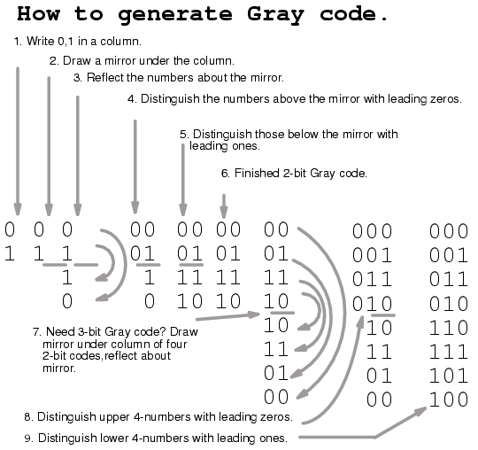
Note that the Gray code sequence, above right, only varies by one bit as we go down the list, or bottom to top up the list. This property of Gray code is often useful for digital electronics in general. In particular, it is applicable to Karnaugh maps.
Examples of Simplification with Karnaugh Maps
Let us move on to some examples of simplification with 3-variable Karnaugh maps. We show how to map the product terms of the unsimplified logic to the K-map. We illustrate how to identify groups of adjacent cells which leads to a Sum-of-Products simplification of the digital logic.
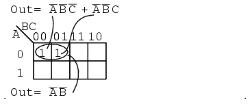
Above we, place the 1’s in the K-map for each of the product terms, identify a group of two, then write a p-term (product term) for the sole group as our simplified result.
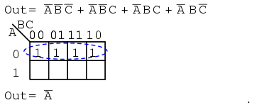
Mapping the four product terms above yields a group of four covered by Boolean A’
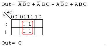
Mapping the four p-terms yields a group of four, which is covered by one variable C.
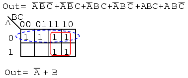
After mapping the six p-terms above, identify the upper group of four, pick up the lower two cells as a group of four by sharing the two with two more from the other group. Covering these two with a group of four gives a simpler result. Since there are two groups, there will be two p-terms in the Sum-of-Products result A’+B
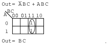
The two product terms above form one group of two and simplifies to BC
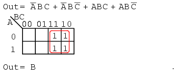
Mapping the four p-terms yields a single group of four, which is B
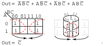
Mapping the four p-terms above yields a group of four. Visualize the group of four by rolling up the ends of the map to form a cylinder, then the cells are adjacent. We normally mark the group of four as above left. Out of the variables A, B, C, there is a common variable: C’. C’ is a 0 overall four cells. The final result is C’.
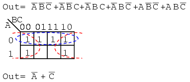
The six cells above from the unsimplified equation can be organized into two groups of four. These two groups should give us two p-terms in our simplified result of A’ + C’.
Simplifying Boolean Equations with Karnaugh Maps
Below, we revisit the toxic waste incinerator from the Boolean algebra chapter. See Boolean algebra chapter for details on this example. We will simplify the logic using a Karnaugh map.
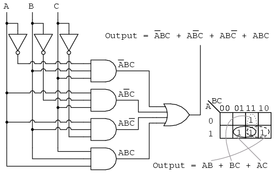
The Boolean equation for the output has four product terms. Map four 1’s corresponding to the p-terms. Forming groups of cells, we have three groups of two. There will be three p-terms in the simplified result, one for each group. See Converting Truth Tables into Boolean Expressions from chapter 7 for a gate diagram of the result, which is reproduced below.
.png?revision=1)
Below we repeat the Boolean algebra simplification of the toxic waste incinerator for comparison.
.png?revision=1)
Below we repeat the Toxic waste incinerator Karnaugh map solution for comparison to the above Boolean algebra simplification. This case illustrates why the Karnaugh map is widely used for logic simplification.

The Karnaugh map method certainly looks easier than the previous pages of Boolean algebra.


