8.7: Larger 4-variable Karnaugh Maps
- Page ID
- 1950
\( \newcommand{\vecs}[1]{\overset { \scriptstyle \rightharpoonup} {\mathbf{#1}} } \)
\( \newcommand{\vecd}[1]{\overset{-\!-\!\rightharpoonup}{\vphantom{a}\smash {#1}}} \)
\( \newcommand{\id}{\mathrm{id}}\) \( \newcommand{\Span}{\mathrm{span}}\)
( \newcommand{\kernel}{\mathrm{null}\,}\) \( \newcommand{\range}{\mathrm{range}\,}\)
\( \newcommand{\RealPart}{\mathrm{Re}}\) \( \newcommand{\ImaginaryPart}{\mathrm{Im}}\)
\( \newcommand{\Argument}{\mathrm{Arg}}\) \( \newcommand{\norm}[1]{\| #1 \|}\)
\( \newcommand{\inner}[2]{\langle #1, #2 \rangle}\)
\( \newcommand{\Span}{\mathrm{span}}\)
\( \newcommand{\id}{\mathrm{id}}\)
\( \newcommand{\Span}{\mathrm{span}}\)
\( \newcommand{\kernel}{\mathrm{null}\,}\)
\( \newcommand{\range}{\mathrm{range}\,}\)
\( \newcommand{\RealPart}{\mathrm{Re}}\)
\( \newcommand{\ImaginaryPart}{\mathrm{Im}}\)
\( \newcommand{\Argument}{\mathrm{Arg}}\)
\( \newcommand{\norm}[1]{\| #1 \|}\)
\( \newcommand{\inner}[2]{\langle #1, #2 \rangle}\)
\( \newcommand{\Span}{\mathrm{span}}\) \( \newcommand{\AA}{\unicode[.8,0]{x212B}}\)
\( \newcommand{\vectorA}[1]{\vec{#1}} % arrow\)
\( \newcommand{\vectorAt}[1]{\vec{\text{#1}}} % arrow\)
\( \newcommand{\vectorB}[1]{\overset { \scriptstyle \rightharpoonup} {\mathbf{#1}} } \)
\( \newcommand{\vectorC}[1]{\textbf{#1}} \)
\( \newcommand{\vectorD}[1]{\overrightarrow{#1}} \)
\( \newcommand{\vectorDt}[1]{\overrightarrow{\text{#1}}} \)
\( \newcommand{\vectE}[1]{\overset{-\!-\!\rightharpoonup}{\vphantom{a}\smash{\mathbf {#1}}}} \)
\( \newcommand{\vecs}[1]{\overset { \scriptstyle \rightharpoonup} {\mathbf{#1}} } \)
\( \newcommand{\vecd}[1]{\overset{-\!-\!\rightharpoonup}{\vphantom{a}\smash {#1}}} \)
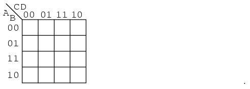
\(\newcommand{\avec}{\mathbf a}\) \(\newcommand{\bvec}{\mathbf b}\) \(\newcommand{\cvec}{\mathbf c}\) \(\newcommand{\dvec}{\mathbf d}\) \(\newcommand{\dtil}{\widetilde{\mathbf d}}\) \(\newcommand{\evec}{\mathbf e}\) \(\newcommand{\fvec}{\mathbf f}\) \(\newcommand{\nvec}{\mathbf n}\) \(\newcommand{\pvec}{\mathbf p}\) \(\newcommand{\qvec}{\mathbf q}\) \(\newcommand{\svec}{\mathbf s}\) \(\newcommand{\tvec}{\mathbf t}\) \(\newcommand{\uvec}{\mathbf u}\) \(\newcommand{\vvec}{\mathbf v}\) \(\newcommand{\wvec}{\mathbf w}\) \(\newcommand{\xvec}{\mathbf x}\) \(\newcommand{\yvec}{\mathbf y}\) \(\newcommand{\zvec}{\mathbf z}\) \(\newcommand{\rvec}{\mathbf r}\) \(\newcommand{\mvec}{\mathbf m}\) \(\newcommand{\zerovec}{\mathbf 0}\) \(\newcommand{\onevec}{\mathbf 1}\) \(\newcommand{\real}{\mathbb R}\) \(\newcommand{\twovec}[2]{\left[\begin{array}{r}#1 \\ #2 \end{array}\right]}\) \(\newcommand{\ctwovec}[2]{\left[\begin{array}{c}#1 \\ #2 \end{array}\right]}\) \(\newcommand{\threevec}[3]{\left[\begin{array}{r}#1 \\ #2 \\ #3 \end{array}\right]}\) \(\newcommand{\cthreevec}[3]{\left[\begin{array}{c}#1 \\ #2 \\ #3 \end{array}\right]}\) \(\newcommand{\fourvec}[4]{\left[\begin{array}{r}#1 \\ #2 \\ #3 \\ #4 \end{array}\right]}\) \(\newcommand{\cfourvec}[4]{\left[\begin{array}{c}#1 \\ #2 \\ #3 \\ #4 \end{array}\right]}\) \(\newcommand{\fivevec}[5]{\left[\begin{array}{r}#1 \\ #2 \\ #3 \\ #4 \\ #5 \\ \end{array}\right]}\) \(\newcommand{\cfivevec}[5]{\left[\begin{array}{c}#1 \\ #2 \\ #3 \\ #4 \\ #5 \\ \end{array}\right]}\) \(\newcommand{\mattwo}[4]{\left[\begin{array}{rr}#1 \amp #2 \\ #3 \amp #4 \\ \end{array}\right]}\) \(\newcommand{\laspan}[1]{\text{Span}\{#1\}}\) \(\newcommand{\bcal}{\cal B}\) \(\newcommand{\ccal}{\cal C}\) \(\newcommand{\scal}{\cal S}\) \(\newcommand{\wcal}{\cal W}\) \(\newcommand{\ecal}{\cal E}\) \(\newcommand{\coords}[2]{\left\{#1\right\}_{#2}}\) \(\newcommand{\gray}[1]{\color{gray}{#1}}\) \(\newcommand{\lgray}[1]{\color{lightgray}{#1}}\) \(\newcommand{\rank}{\operatorname{rank}}\) \(\newcommand{\row}{\text{Row}}\) \(\newcommand{\col}{\text{Col}}\) \(\renewcommand{\row}{\text{Row}}\) \(\newcommand{\nul}{\text{Nul}}\) \(\newcommand{\var}{\text{Var}}\) \(\newcommand{\corr}{\text{corr}}\) \(\newcommand{\len}[1]{\left|#1\right|}\) \(\newcommand{\bbar}{\overline{\bvec}}\) \(\newcommand{\bhat}{\widehat{\bvec}}\) \(\newcommand{\bperp}{\bvec^\perp}\) \(\newcommand{\xhat}{\widehat{\xvec}}\) \(\newcommand{\vhat}{\widehat{\vvec}}\) \(\newcommand{\uhat}{\widehat{\uvec}}\) \(\newcommand{\what}{\widehat{\wvec}}\) \(\newcommand{\Sighat}{\widehat{\Sigma}}\) \(\newcommand{\lt}{<}\) \(\newcommand{\gt}{>}\) \(\newcommand{\amp}{&}\) \(\definecolor{fillinmathshade}{gray}{0.9}\)Knowing how to generate Gray code should allow us to build larger maps. Actually, all we need to do is look at the left to right sequence across the top of the 3-variable map, and copy it down the left side of the 4-variable map. See below.
Reductions of 4 Variable K Maps
The following four variable Karnaugh maps illustrate the reduction of Boolean expressions too tedious for Boolean algebra. Reductions could be done with Boolean algebra. However, the Karnaugh map is faster and easier, especially if there are many logic reductions to do.
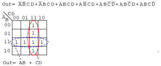
The above Boolean expression has seven product terms. They are mapped top to bottom and left to right on the K-map above. For example, the first P-term A’B’CD is the first row, 3rd cell, corresponding to map location A=0, B=0, C=1, D=1. The other product terms are placed in a similar manner. Encircling the largest groups possible, two groups of four are shown above. The dashed horizontal group corresponds to the simplified product term AB. The vertical group corresponds to Boolean CD. Since there are two groups, there will be two product terms in the Sum-Of-Products result of Out=AB+CD.
Fold up the corners of the map below like it is a napkin to make the four cells physically adjacent.
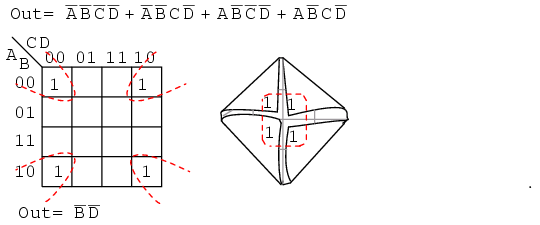
The four cells above are a group of four because they all have the Boolean variables B’ and D’ in common. In other words, B=0 for the four cells, and D=0 for the four cells. The other variables (A, C) are 0 in some cases, 1 in other cases with respect to the four corner cells. Thus, these variables (A, C) are not involved with this group of four. This single group comes out of the map as one product term for the simplified result: Out=B’D’
For the K-map below, roll the top and bottom edges into a cylinder forming eight adjacent cells.
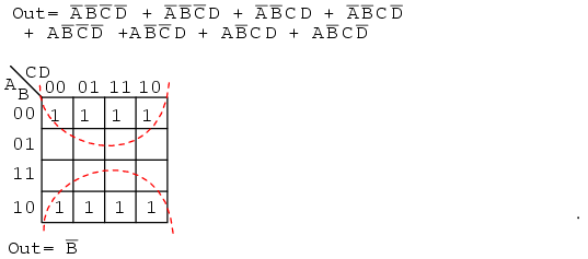
The above group of eight has one Boolean variable in common: B=0. Therefore, the one group of eight is covered by one p-term: B’. The original eight-term Boolean expression simplifies to Out=B’
P-Terms in 4 Variable K Maps
The Boolean expression below has nine p-terms, three of which have three Booleans instead of four. The difference is that while four Boolean variable product terms cover one cell, the three Boolean p-terms cover a pair of cells each.
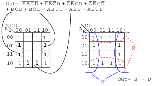
The six product terms of four Boolean variables map in the usual manner above as single cells. The three Boolean variable terms (three each) map as cell pairs, which is shown above. Note that we are mapping p-terms into the K-map, not pulling them out at this point.
For the simplification, we form two groups of eight. Cells in the corners are shared with both groups. This is fine. In fact, this leads to a better solution than forming a group of eight and a group of four without sharing any cells. Final Solution is Out=B’+D’
Below we map the unsimplified Boolean expression to the Karnaugh map.
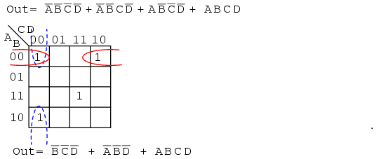
Above, three of the cells form into groups of two cells. A fourth cell cannot be combined with anything, which often happens in “real world” problems. In this case, the Boolean p-term ABCD is unchanged in the simplification process. Result: Out= B’C’D’+A’B’D’+ABCD
Often times there is more than one minimum cost solution to a simplification problem. Such is the case illustrated below.
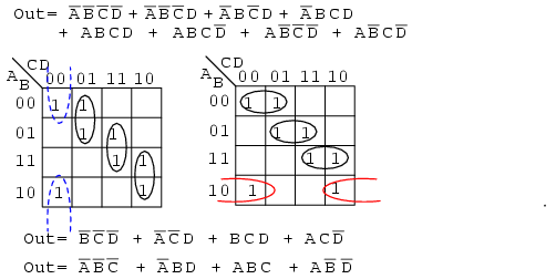
Both results above have four product terms of three Boolean variable each. Both are equally valid minimal cost solutions. The difference in the final solution is due to how the cells are grouped as shown above. A minimal cost solution is a valid logic design with the minimum number of gates with the minimum number of inputs.
Below we map the unsimplified Boolean equation as usual and form a group of four as a first simplification step. It may not be obvious how to pick up the remaining cells.
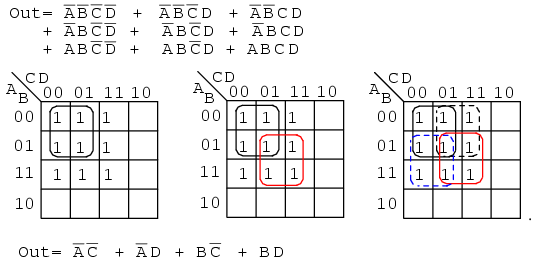
Pick up three more cells in a group of four, center above. There are still two cells remaining. the minimal cost method to pick up those is to group them with neighboring cells as groups of four as at above right.
On a cautionary note, do not attempt to form groups of three. Groupings must be powers of 2, that is, 1, 2, 4, 8 ...
Below we have another example of two possible minimal cost solutions. Start by forming a couple of groups of four after mapping the cells.
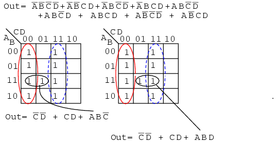
The two solutions depend on whether the single remaining cell is grouped with the first or the second group of four as a group of two cells. That cell either comes out as either ABC’ or ABD, your choice. Either way, this cell is covered by either Boolean product term. Final results are shown above.
Below we have an example of a simplification using the Karnaugh map at left or Boolean algebra at right. Plot C’ on the map as the area of all cells covered by address C=0, the 8-cells on the left of the map. Then, plot the single ABCD cell. That single cell forms a group of 2-cell as shown, which simplifies to P-term ABD, for an end result of Out = C’ + ABD.
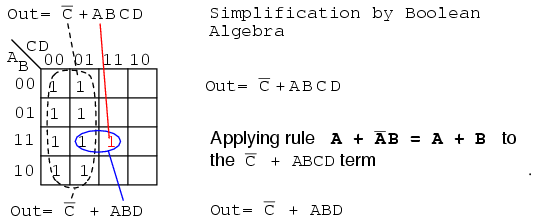
This (above) is a rare example of a four-variable problem that can be reduced with Boolean algebra without a lot of work, assuming that you remember the theorems.


