6.4: Derivatives of Power Functions of e

Last updated
Save as PDF

Page ID: 1117

$ \newcommand{\vecs}[1]{\overset { \scriptstyle \rightharpoonup} {\mathbf{#1}} } $ $ \newcommand{\vecd}[1]{\overset{-\!-\!\rightharpoonup}{\vphantom{a}\smash {#1}}} $$\newcommand{\id}{\mathrm{id}}$ $ \newcommand{\Span}{\mathrm{span}}$ $ \newcommand{\kernel}{\mathrm{null}\,}$ $ \newcommand{\range}{\mathrm{range}\,}$ $ \newcommand{\RealPart}{\mathrm{Re}}$ $ \newcommand{\ImaginaryPart}{\mathrm{Im}}$ $ \newcommand{\Argument}{\mathrm{Arg}}$ $ \newcommand{\norm}[1]{\| #1 \|}$ $ \newcommand{\inner}[2]{\langle #1, #2 \rangle}$ $ \newcommand{\Span}{\mathrm{span}}$ $\newcommand{\id}{\mathrm{id}}$ $ \newcommand{\Span}{\mathrm{span}}$ $ \newcommand{\kernel}{\mathrm{null}\,}$ $ \newcommand{\range}{\mathrm{range}\,}$ $ \newcommand{\RealPart}{\mathrm{Re}}$ $ \newcommand{\ImaginaryPart}{\mathrm{Im}}$ $ \newcommand{\Argument}{\mathrm{Arg}}$ $ \newcommand{\norm}[1]{\| #1 \|}$ $ \newcommand{\inner}[2]{\langle #1, #2 \rangle}$ $ \newcommand{\Span}{\mathrm{span}}$$\newcommand{\AA}{\unicode[.8,0]{x212B}}$

Example Derivatives of e

Proportionality Constant

When we say that a relationship or phenomenon is “exponential,” we are implying that some quantity—electric current, profits, population—increases more rapidly as the quantity grows. In other words, the rate of change with respect to a given variable is proportional to the value of that variable. This means that the derivative of an exponential function is equal to the original exponential function multiplied by a constant (k) that establishes proportionality.

The proportionality constant is equal to the natural log of the base of the exponent:

It follows, then, that if the natural log of the base is equal to one, the derivative of the function will be equal to the original function. This is exactly what happens with power functions of e: the natural log of e is 1, and consequently, the derivative of e^x is e^x.

The “Chain” Rule

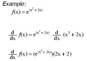
When the exponential expression is something other than simply x, we apply the chain rule: First we take the derivative of the entire expression, then we multiply it by the derivative of the expression in the exponent.

This technique can be used to find the rate of change of diode current with respect to diode voltage.

The following equation provides an approximate relationship between the voltage across a diode ($V_D$)and the current through a diode($I_D$):

(See the page on diodes and rectifiers for more information on the diode current–voltage equation; also, note that ($I_S$) is a constant, not a variable.) To find the rate of change of current with respect to voltage, we take the derivative:

Thus, at a given value of diode voltage ($V_D$) , an incremental increase in voltage will create an increase in current equal to $$\frac{I_S}{0.026}e^\frac{V_D}{0.026}\]