
5.4: Series-parallel R, L, and C
- Page ID
- 1410

\( \newcommand{\vecs}[1]{\overset { \scriptstyle \rightharpoonup} {\mathbf{#1}} } \)
\( \newcommand{\vecd}[1]{\overset{-\!-\!\rightharpoonup}{\vphantom{a}\smash {#1}}} \)
\( \newcommand{\dsum}{\displaystyle\sum\limits} \)
\( \newcommand{\dint}{\displaystyle\int\limits} \)
\( \newcommand{\dlim}{\displaystyle\lim\limits} \)
\( \newcommand{\id}{\mathrm{id}}\) \( \newcommand{\Span}{\mathrm{span}}\)
( \newcommand{\kernel}{\mathrm{null}\,}\) \( \newcommand{\range}{\mathrm{range}\,}\)
\( \newcommand{\RealPart}{\mathrm{Re}}\) \( \newcommand{\ImaginaryPart}{\mathrm{Im}}\)
\( \newcommand{\Argument}{\mathrm{Arg}}\) \( \newcommand{\norm}[1]{\| #1 \|}\)
\( \newcommand{\inner}[2]{\langle #1, #2 \rangle}\)
\( \newcommand{\Span}{\mathrm{span}}\)
\( \newcommand{\id}{\mathrm{id}}\)
\( \newcommand{\Span}{\mathrm{span}}\)
\( \newcommand{\kernel}{\mathrm{null}\,}\)
\( \newcommand{\range}{\mathrm{range}\,}\)
\( \newcommand{\RealPart}{\mathrm{Re}}\)
\( \newcommand{\ImaginaryPart}{\mathrm{Im}}\)
\( \newcommand{\Argument}{\mathrm{Arg}}\)
\( \newcommand{\norm}[1]{\| #1 \|}\)
\( \newcommand{\inner}[2]{\langle #1, #2 \rangle}\)
\( \newcommand{\Span}{\mathrm{span}}\) \( \newcommand{\AA}{\unicode[.8,0]{x212B}}\)
\( \newcommand{\vectorA}[1]{\vec{#1}} % arrow\)
\( \newcommand{\vectorAt}[1]{\vec{\text{#1}}} % arrow\)
\( \newcommand{\vectorB}[1]{\overset { \scriptstyle \rightharpoonup} {\mathbf{#1}} } \)
\( \newcommand{\vectorC}[1]{\textbf{#1}} \)
\( \newcommand{\vectorD}[1]{\overrightarrow{#1}} \)
\( \newcommand{\vectorDt}[1]{\overrightarrow{\text{#1}}} \)
\( \newcommand{\vectE}[1]{\overset{-\!-\!\rightharpoonup}{\vphantom{a}\smash{\mathbf {#1}}}} \)
\( \newcommand{\vecs}[1]{\overset { \scriptstyle \rightharpoonup} {\mathbf{#1}} } \)
\(\newcommand{\longvect}{\overrightarrow}\)
\( \newcommand{\vecd}[1]{\overset{-\!-\!\rightharpoonup}{\vphantom{a}\smash {#1}}} \)
\(\newcommand{\avec}{\mathbf a}\) \(\newcommand{\bvec}{\mathbf b}\) \(\newcommand{\cvec}{\mathbf c}\) \(\newcommand{\dvec}{\mathbf d}\) \(\newcommand{\dtil}{\widetilde{\mathbf d}}\) \(\newcommand{\evec}{\mathbf e}\) \(\newcommand{\fvec}{\mathbf f}\) \(\newcommand{\nvec}{\mathbf n}\) \(\newcommand{\pvec}{\mathbf p}\) \(\newcommand{\qvec}{\mathbf q}\) \(\newcommand{\svec}{\mathbf s}\) \(\newcommand{\tvec}{\mathbf t}\) \(\newcommand{\uvec}{\mathbf u}\) \(\newcommand{\vvec}{\mathbf v}\) \(\newcommand{\wvec}{\mathbf w}\) \(\newcommand{\xvec}{\mathbf x}\) \(\newcommand{\yvec}{\mathbf y}\) \(\newcommand{\zvec}{\mathbf z}\) \(\newcommand{\rvec}{\mathbf r}\) \(\newcommand{\mvec}{\mathbf m}\) \(\newcommand{\zerovec}{\mathbf 0}\) \(\newcommand{\onevec}{\mathbf 1}\) \(\newcommand{\real}{\mathbb R}\) \(\newcommand{\twovec}[2]{\left[\begin{array}{r}#1 \\ #2 \end{array}\right]}\) \(\newcommand{\ctwovec}[2]{\left[\begin{array}{c}#1 \\ #2 \end{array}\right]}\) \(\newcommand{\threevec}[3]{\left[\begin{array}{r}#1 \\ #2 \\ #3 \end{array}\right]}\) \(\newcommand{\cthreevec}[3]{\left[\begin{array}{c}#1 \\ #2 \\ #3 \end{array}\right]}\) \(\newcommand{\fourvec}[4]{\left[\begin{array}{r}#1 \\ #2 \\ #3 \\ #4 \end{array}\right]}\) \(\newcommand{\cfourvec}[4]{\left[\begin{array}{c}#1 \\ #2 \\ #3 \\ #4 \end{array}\right]}\) \(\newcommand{\fivevec}[5]{\left[\begin{array}{r}#1 \\ #2 \\ #3 \\ #4 \\ #5 \\ \end{array}\right]}\) \(\newcommand{\cfivevec}[5]{\left[\begin{array}{c}#1 \\ #2 \\ #3 \\ #4 \\ #5 \\ \end{array}\right]}\) \(\newcommand{\mattwo}[4]{\left[\begin{array}{rr}#1 \amp #2 \\ #3 \amp #4 \\ \end{array}\right]}\) \(\newcommand{\laspan}[1]{\text{Span}\{#1\}}\) \(\newcommand{\bcal}{\cal B}\) \(\newcommand{\ccal}{\cal C}\) \(\newcommand{\scal}{\cal S}\) \(\newcommand{\wcal}{\cal W}\) \(\newcommand{\ecal}{\cal E}\) \(\newcommand{\coords}[2]{\left\{#1\right\}_{#2}}\) \(\newcommand{\gray}[1]{\color{gray}{#1}}\) \(\newcommand{\lgray}[1]{\color{lightgray}{#1}}\) \(\newcommand{\rank}{\operatorname{rank}}\) \(\newcommand{\row}{\text{Row}}\) \(\newcommand{\col}{\text{Col}}\) \(\renewcommand{\row}{\text{Row}}\) \(\newcommand{\nul}{\text{Nul}}\) \(\newcommand{\var}{\text{Var}}\) \(\newcommand{\corr}{\text{corr}}\) \(\newcommand{\len}[1]{\left|#1\right|}\) \(\newcommand{\bbar}{\overline{\bvec}}\) \(\newcommand{\bhat}{\widehat{\bvec}}\) \(\newcommand{\bperp}{\bvec^\perp}\) \(\newcommand{\xhat}{\widehat{\xvec}}\) \(\newcommand{\vhat}{\widehat{\vvec}}\) \(\newcommand{\uhat}{\widehat{\uvec}}\) \(\newcommand{\what}{\widehat{\wvec}}\) \(\newcommand{\Sighat}{\widehat{\Sigma}}\) \(\newcommand{\lt}{<}\) \(\newcommand{\gt}{>}\) \(\newcommand{\amp}{&}\) \(\definecolor{fillinmathshade}{gray}{0.9}\)Now that we’ve seen how series and parallel AC circuit analysis is not fundamentally different than DC circuit analysis, it should come as no surprise that series-parallel analysis would be the same as well, just using complex numbers instead of scalar to represent voltage, current, and impedance.
Take this series-parallel circuit for example: (Figure below)
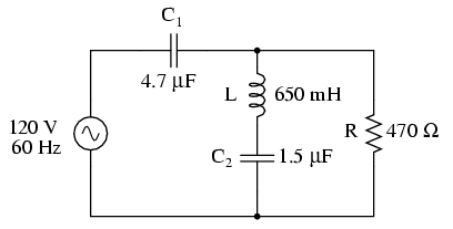
Example series-parallel R, L, and C circuit.
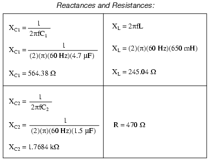
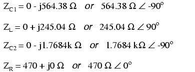
The first order of business, as usual, is to determine values of impedance (Z) for all components based on the frequency of the AC power source. To do this, we need to first determine values of reactance (X) for all inductors and capacitors, then convert reactance (X) and resistance (R) figures into proper impedance (Z) form:
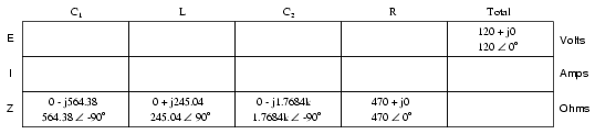
Now we can set up the initial values in our table:
Being a series-parallel combination circuit, we must reduce it to a total impedance in more than one step. The first step is to combine L and C2 as a series combination of impedances, by adding their impedances together. Then, that impedance will be combined in parallel with the impedance of the resistor, to arrive at another combination of impedances. Finally, that quantity will be added to the impedance of C1 to arrive at the total impedance.
In order that our table may follow all these steps, it will be necessary to add additional columns to it so that each step may be represented. Adding more columns horizontally to the table shown above would be impractical for formatting reasons, so I will place a new row of columns underneath, each column designated by its respective component combination:
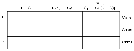
Calculating these new (combination) impedances will require complex addition for series combinations, and the “reciprocal” formula for complex impedances in parallel. This time, there is no avoidance of the reciprocal formula: the required figures can be arrived at no other way!
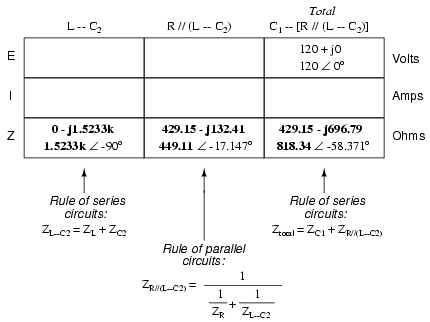
Seeing as how our second table contains a column for “Total,” we can safely discard that column from the first table. This gives us one table with four columns and another table with three columns.
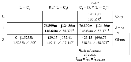
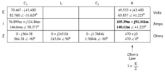
Now that we know the total impedance (818.34 Ω ∠ -58.371o) and the total voltage (120 volts ∠ 0o), we can apply Ohm’s Law (I=E/Z) vertically in the “Total” column to arrive at a figure for total current:
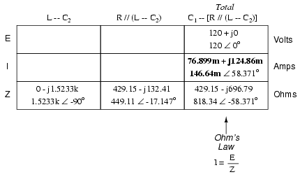
At this point we ask ourselves the question: are there any components or component combinations which share either the total voltage or the total current? In this case, both C1 and the parallel combination R//(L—C2) share the same (total) current, since the total impedance is composed of the two sets of impedances in series. Thus, we can transfer the figure for total current into both columns:
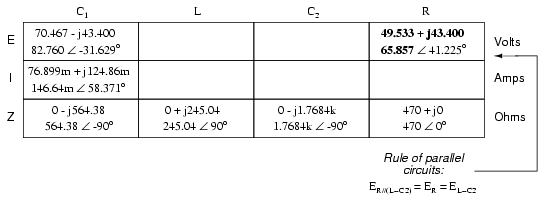
Now, we can calculate voltage drops across C1 and the series-parallel combination of R//(L—C2) using Ohm’s Law (E=IZ) vertically in those table columns:
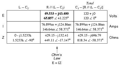
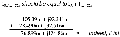
A quick double-check of our work at this point would be to see whether or not the voltage drops across C1and the series-parallel combination of R//(L—C2) indeed add up to the total. According to Kirchhoff’s Voltage Law, they should!
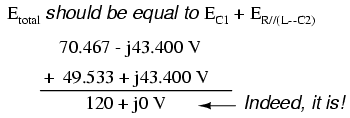
That last step was merely a precaution. In a problem with as many steps as this one has, there is much opportunity for error. Occasional cross-checks like that one can save a person a lot of work and unnecessary frustration by identifying problems prior to the final step of the problem.
After having solved for voltage drops across C1 and the combination R//(L—C2), we again ask ourselves the question: what other components share the same voltage or current? In this case, the resistor (R) and the combination of the inductor and the second capacitor (L—C2) share the same voltage, because those sets of impedances are in parallel with each other. Therefore, we can transfer the voltage figure just solved for into the columns for R and L—C2:
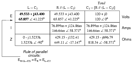
Now we’re all set for calculating current through the resistor and through the series combination L—C2. All we need to do is apply Ohm’s Law (I=E/Z) vertically in both of those columns:
Another quick double-check of our work at this point would be to see if the current figures for L—C2 and R add up to the total current. According to Kirchhoff’s Current Law, they should:
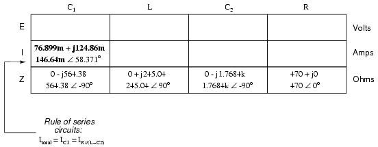
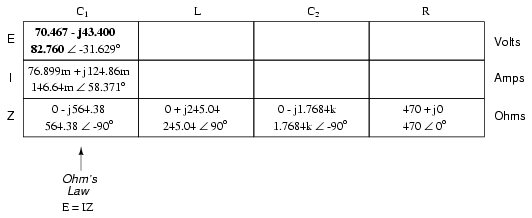
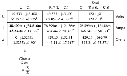
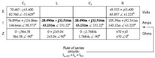
Since the L and C2 are connected in series, and since we know the current through their series combination impedance, we can distribute that current figure to the L and C2 columns following the rule of series circuits whereby series components share the same current:
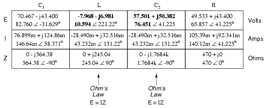
With one last step (actually, two calculations), we can complete our analysis table for this circuit. With impedance and current figures in place for L and C2, all we have to do is apply Ohm’s Law (E=IZ) vertically in those two columns to calculate voltage drops.
Now, let’s turn to SPICE for a computer verification of our work:
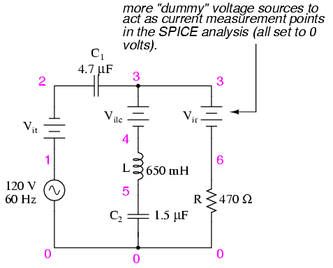
Example series-parallel R, L, C SPICE circuit.
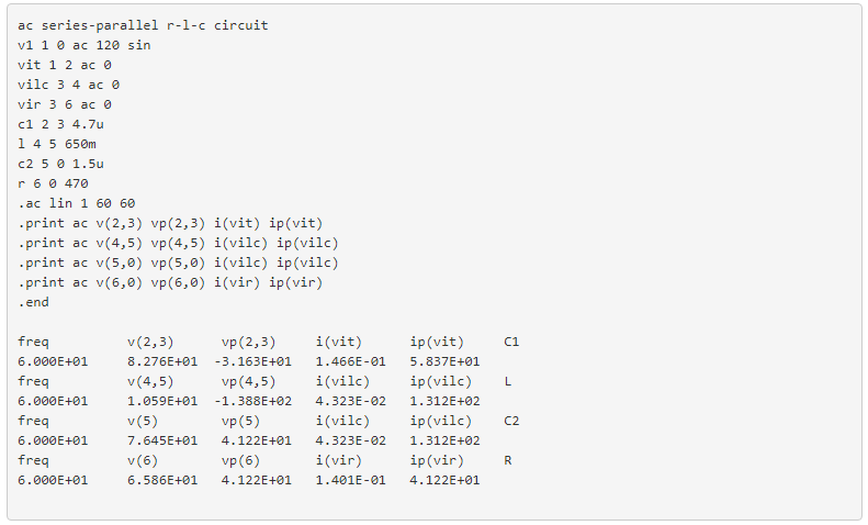
Each line of the SPICE output listing gives the voltage, voltage phase angle, current, and current phase angle for C1, L, C2, and R, in that order. As you can see, these figures do concur with our hand-calculated figures in the circuit analysis table.
As daunting a task as series-parallel AC circuit analysis may appear, it must be emphasized that there is nothing really new going on here besides the use of complex numbers. Ohm’s Law (in its new form of E=IZ) still holds true, as do the voltage and current Laws of Kirchhoff. While there is more potential for human error in carrying out the necessary complex number calculations, the basic principles and techniques of series-parallel circuit reduction are exactly the same.
Review
- Analysis of series-parallel AC circuits is much the same as series-parallel DC circuits. The only substantive difference is that all figures and calculations are in complex (not scalar) form.
- It is important to remember that before series-parallel reduction (simplification) can begin, you must determine the impedance (Z) of every resistor, inductor, and capacitor. That way, all component values will be expressed in common terms (Z) instead of an incompatible mix of resistance (R), inductance (L), and capacitance (C).