
2.3: Functions for Personal Finance
- Page ID
- 14401

\( \newcommand{\vecs}[1]{\overset { \scriptstyle \rightharpoonup} {\mathbf{#1}} } \)
\( \newcommand{\vecd}[1]{\overset{-\!-\!\rightharpoonup}{\vphantom{a}\smash {#1}}} \)
\( \newcommand{\dsum}{\displaystyle\sum\limits} \)
\( \newcommand{\dint}{\displaystyle\int\limits} \)
\( \newcommand{\dlim}{\displaystyle\lim\limits} \)
\( \newcommand{\id}{\mathrm{id}}\) \( \newcommand{\Span}{\mathrm{span}}\)
( \newcommand{\kernel}{\mathrm{null}\,}\) \( \newcommand{\range}{\mathrm{range}\,}\)
\( \newcommand{\RealPart}{\mathrm{Re}}\) \( \newcommand{\ImaginaryPart}{\mathrm{Im}}\)
\( \newcommand{\Argument}{\mathrm{Arg}}\) \( \newcommand{\norm}[1]{\| #1 \|}\)
\( \newcommand{\inner}[2]{\langle #1, #2 \rangle}\)
\( \newcommand{\Span}{\mathrm{span}}\)
\( \newcommand{\id}{\mathrm{id}}\)
\( \newcommand{\Span}{\mathrm{span}}\)
\( \newcommand{\kernel}{\mathrm{null}\,}\)
\( \newcommand{\range}{\mathrm{range}\,}\)
\( \newcommand{\RealPart}{\mathrm{Re}}\)
\( \newcommand{\ImaginaryPart}{\mathrm{Im}}\)
\( \newcommand{\Argument}{\mathrm{Arg}}\)
\( \newcommand{\norm}[1]{\| #1 \|}\)
\( \newcommand{\inner}[2]{\langle #1, #2 \rangle}\)
\( \newcommand{\Span}{\mathrm{span}}\) \( \newcommand{\AA}{\unicode[.8,0]{x212B}}\)
\( \newcommand{\vectorA}[1]{\vec{#1}} % arrow\)
\( \newcommand{\vectorAt}[1]{\vec{\text{#1}}} % arrow\)
\( \newcommand{\vectorB}[1]{\overset { \scriptstyle \rightharpoonup} {\mathbf{#1}} } \)
\( \newcommand{\vectorC}[1]{\textbf{#1}} \)
\( \newcommand{\vectorD}[1]{\overrightarrow{#1}} \)
\( \newcommand{\vectorDt}[1]{\overrightarrow{\text{#1}}} \)
\( \newcommand{\vectE}[1]{\overset{-\!-\!\rightharpoonup}{\vphantom{a}\smash{\mathbf {#1}}}} \)
\( \newcommand{\vecs}[1]{\overset { \scriptstyle \rightharpoonup} {\mathbf{#1}} } \)
\(\newcommand{\longvect}{\overrightarrow}\)
\( \newcommand{\vecd}[1]{\overset{-\!-\!\rightharpoonup}{\vphantom{a}\smash {#1}}} \)
\(\newcommand{\avec}{\mathbf a}\) \(\newcommand{\bvec}{\mathbf b}\) \(\newcommand{\cvec}{\mathbf c}\) \(\newcommand{\dvec}{\mathbf d}\) \(\newcommand{\dtil}{\widetilde{\mathbf d}}\) \(\newcommand{\evec}{\mathbf e}\) \(\newcommand{\fvec}{\mathbf f}\) \(\newcommand{\nvec}{\mathbf n}\) \(\newcommand{\pvec}{\mathbf p}\) \(\newcommand{\qvec}{\mathbf q}\) \(\newcommand{\svec}{\mathbf s}\) \(\newcommand{\tvec}{\mathbf t}\) \(\newcommand{\uvec}{\mathbf u}\) \(\newcommand{\vvec}{\mathbf v}\) \(\newcommand{\wvec}{\mathbf w}\) \(\newcommand{\xvec}{\mathbf x}\) \(\newcommand{\yvec}{\mathbf y}\) \(\newcommand{\zvec}{\mathbf z}\) \(\newcommand{\rvec}{\mathbf r}\) \(\newcommand{\mvec}{\mathbf m}\) \(\newcommand{\zerovec}{\mathbf 0}\) \(\newcommand{\onevec}{\mathbf 1}\) \(\newcommand{\real}{\mathbb R}\) \(\newcommand{\twovec}[2]{\left[\begin{array}{r}#1 \\ #2 \end{array}\right]}\) \(\newcommand{\ctwovec}[2]{\left[\begin{array}{c}#1 \\ #2 \end{array}\right]}\) \(\newcommand{\threevec}[3]{\left[\begin{array}{r}#1 \\ #2 \\ #3 \end{array}\right]}\) \(\newcommand{\cthreevec}[3]{\left[\begin{array}{c}#1 \\ #2 \\ #3 \end{array}\right]}\) \(\newcommand{\fourvec}[4]{\left[\begin{array}{r}#1 \\ #2 \\ #3 \\ #4 \end{array}\right]}\) \(\newcommand{\cfourvec}[4]{\left[\begin{array}{c}#1 \\ #2 \\ #3 \\ #4 \end{array}\right]}\) \(\newcommand{\fivevec}[5]{\left[\begin{array}{r}#1 \\ #2 \\ #3 \\ #4 \\ #5 \\ \end{array}\right]}\) \(\newcommand{\cfivevec}[5]{\left[\begin{array}{c}#1 \\ #2 \\ #3 \\ #4 \\ #5 \\ \end{array}\right]}\) \(\newcommand{\mattwo}[4]{\left[\begin{array}{rr}#1 \amp #2 \\ #3 \amp #4 \\ \end{array}\right]}\) \(\newcommand{\laspan}[1]{\text{Span}\{#1\}}\) \(\newcommand{\bcal}{\cal B}\) \(\newcommand{\ccal}{\cal C}\) \(\newcommand{\scal}{\cal S}\) \(\newcommand{\wcal}{\cal W}\) \(\newcommand{\ecal}{\cal E}\) \(\newcommand{\coords}[2]{\left\{#1\right\}_{#2}}\) \(\newcommand{\gray}[1]{\color{gray}{#1}}\) \(\newcommand{\lgray}[1]{\color{lightgray}{#1}}\) \(\newcommand{\rank}{\operatorname{rank}}\) \(\newcommand{\row}{\text{Row}}\) \(\newcommand{\col}{\text{Col}}\) \(\renewcommand{\row}{\text{Row}}\) \(\newcommand{\nul}{\text{Nul}}\) \(\newcommand{\var}{\text{Var}}\) \(\newcommand{\corr}{\text{corr}}\) \(\newcommand{\len}[1]{\left|#1\right|}\) \(\newcommand{\bbar}{\overline{\bvec}}\) \(\newcommand{\bhat}{\widehat{\bvec}}\) \(\newcommand{\bperp}{\bvec^\perp}\) \(\newcommand{\xhat}{\widehat{\xvec}}\) \(\newcommand{\vhat}{\widehat{\vvec}}\) \(\newcommand{\uhat}{\widehat{\uvec}}\) \(\newcommand{\what}{\widehat{\wvec}}\) \(\newcommand{\Sighat}{\widehat{\Sigma}}\) \(\newcommand{\lt}{<}\) \(\newcommand{\gt}{>}\) \(\newcommand{\amp}{&}\) \(\definecolor{fillinmathshade}{gray}{0.9}\)Learning Objectives
- Understand the fundamentals of loans.
- Use the PMT function to calculate monthly car loan payments.
- Use the PMT function to calculate monthly mortgage payments on a house using a down payment.
- Learn how to summarize data in a workbook by using worksheet links to create a summary worksheet.
In this section, we continue to develop the Personal Budget workbook. Notable items that are missing from the Budget Detail worksheet are the payments you might make for a car or a home. This section demonstrates Excel functions used to calculate loan payments for a car and to calculate mortgage payments for a house.
The Fundamentals of Loans and Leases
One of the functions we will add to the Personal Budget workbook is the PMT function. This function calculates the payments required for loan repayment. However, before demonstrating this function, it is important to cover a few fundamental concepts on loans.
A loan is a contractual agreement in which money is borrowed from a lender and paid back over a specific period of time. The amount of money that is borrowed from the lender is called the principal of the loan. The borrower is usually required to pay the principal of the loan plus interest. When you borrow money to buy a house, the loan is referred to as a mortgage. This is because the house being purchased also serves as collateral to ensure payment. In other words, the bank can take possession of your house if you fail to make loan payments. As shown in Table 2.5, there are several key terms related to loans.
| Term | Definition |
|---|---|
| Collateral | Any item of value that is used to secure a loan to ensure payments to the lender |
| Down Payment | The amount of cash paid toward the purchase of a house. If you are paying 20% down, you are paying 20% of the cost of the house in cash and are borrowing the rest from a lender. |
| Interest Rate | The interest that is charged to the borrower as a cost for borrowing money |
| Mortgage | A loan where property is put up for collateral |
| Principal | The amount of money that has been borrowed |
| Residual Value | The estimated selling price of a vehicle at a future point in time |
| Length | The amount of time you have to repay a loan |
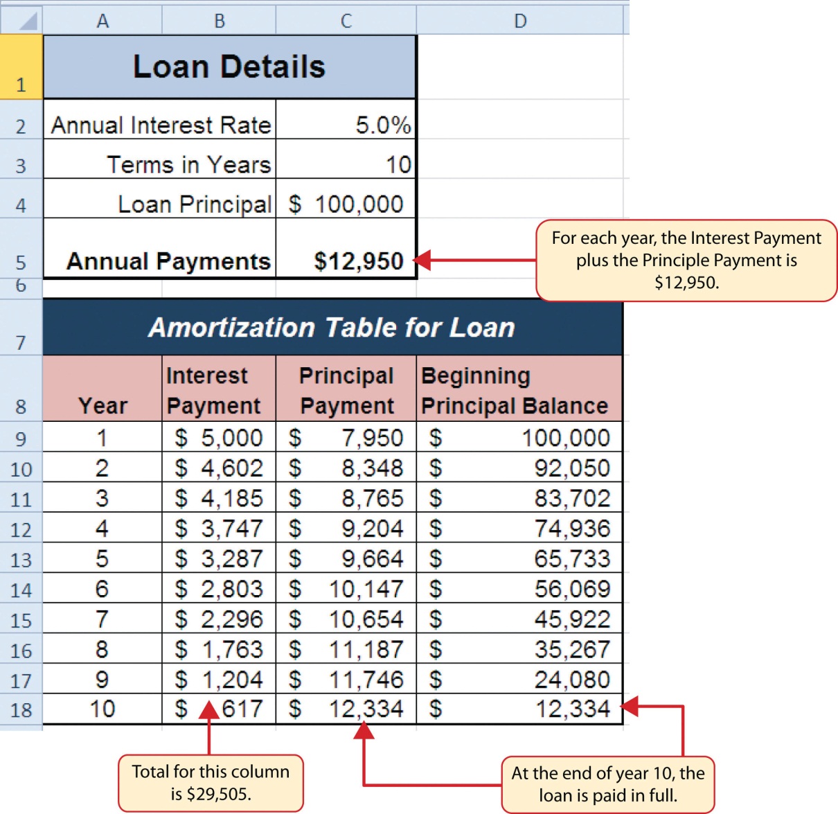
Figure 2.31 shows an example of an amortization table for a loan. A lender is required by law to provide borrowers with an amortization table when a loan contract is offered. The table in the figure shows how the payments of a loan would work if you borrowed $100,000 from a lender and agreed to pay it back over 10 years at an interest rate of 5%. You will notice that each time you make a payment, you are paying the bank an interest fee plus some of the loan principal. Each year the amount of interest paid to the bank decreases and the amount of money used to pay off the principal increases. This is because the bank is charging you interest on the amount of principal that has not been paid. As you pay off the principal, the interest rate is applied to a lower number, which reduces your interest charges. Finally, the figure shows that the sum of the values in the Interest Payment column is $29,505. This is how much it costs you to borrow this money over 10 years. Indeed, borrowing money is not free. It is important to note that to simplify this example, the payments were calculated on an annual basis. However, most loan payments are made on a monthly basis.
The PMT (Payment) Function for Loans
Data file: Continue with CH2 Personal Budget.
If you own a home, your mortgage payments are a major component of your household budget. If you are planning to buy a home, having a clear understanding of your monthly payments is critical for maintaining strong financial health. In Excel, mortgage payments are conveniently calculated through the PMT (payment) function. This function is more complex than the statistical functions covered in Section 2.2 “Statistical Functions”. With statistical functions, you are required to add only a range of cells or selected cells within the parentheses of the function, also known as the argument. With the PMT function, you must accurately define a series of arguments in order for the function to produce a reliable output. Table 2.6 lists the arguments for the PMT function. It is helpful to review the key loan terms in Table 2.5 before reviewing the PMT function arguments.
| Argument | Definition |
|---|---|
| Rate | This is the interest rate the lender is charging the borrower. The interest rate is usually quoted in annual terms, so you have to divide this rate by 12 if you are calculating monthly payments. |
| Nper | The argument letters stand for number of periods. This is the term of the loan, which is the amount of time you have to repay the bank. This is usually quoted in years, so you have to multiply the years by 12 if you are calculating monthly payments. |
| Pv | The argument letters stand for present value. This is the principal of the loan or the amount of money that is borrowed. |
| [Fv] | The argument letters stand for future value. The brackets around the argument indicate that it is not always necessary to define it. It is used if there is a lump-sum payment that will be made at the end of the loan terms. This is also used for the residual value of a lease. If it is not defined, Excel will assume that it is zero. |
| [Type] | This argument can be defined with either a 1 or a 0. The number 1 is used if payments are made at the beginning of each period. A 0 is used if payments are made at the end of each period. The argument is in brackets because it does not have to be defined if payments are made at the end of each period. Excel assumes that this argument is 0 if it is not defined. |
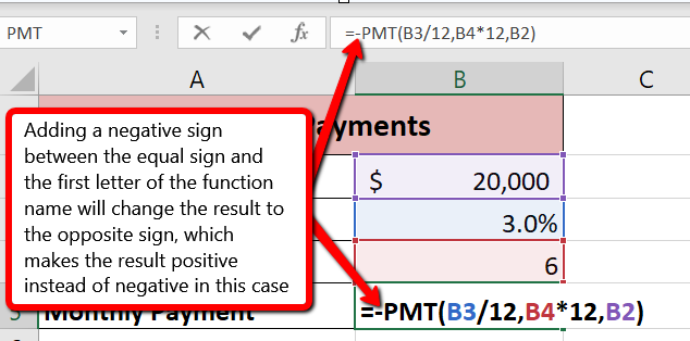
By default, the result of the PMT function in Excel is shown as a negative number. This is because it represents an outgoing payment. When making a mortgage or car payment, you are paying money out of your pocket or bank account. Depending on the type of work that you do, your employer may want you to leave your payments negative or they may ask you to format them as positive numbers. In the following assignments, the payments calculated using the PMT function will be made positive to make them easier to work with. To do this, you will place a negative sign between the equal sign and the function name PMT.
We will first use the PMT function in the Personal Budget workbook to calculate the monthly loan payments for a car. These calculations will be made in the Loan Payments worksheet and then displayed in the Budget Summary worksheet through a cell reference link. So far we have demonstrated several methods for adding functions to a worksheet. When working with more complex functions such as the PMT, it is easiest to use the Function Dialog box.
Remember to use cell references for the arguments of the PMT function whenever possible. This will allow you the flexibility to change aspects of the loan, such as a lower interest rate or more expensive car, and have the payment automatically recalculate.
Using cell references for the arguments provides greater flexibility in trying different scenarios.
The following steps use the Insert Function command covered in Section 2.2 to add the PMT function:
- Switch to the Loan Payments worksheet.
- Click cell B5.
- Click the Formulas tab on the Ribbon.
- Click the Insert Function button to bring up the Insert Function dialog box.
- Type loan payment in the search box and click Go.
 the Excel for Mac search box does is not the same as the “Search for a function: input box”. Mac Users must type: PMT in the search box instead. Then press Enter.
 - Double-click the PMT option in the “Select a function:” box. This will open the Function Arguments dialog box.
- Drag the Function Arguments dialog box out of the way so that you can see the worksheet cells you want to use in the function. Refer to Figure 2.31for the completed Function Arguments dialog box as you complete the next steps.
- Click in the Rate argument box in the dialog box, then click cell B3 in the worksheet. This will add B3 (the annual interest rate) to the Rate argument.
- Type a forward slash / for division.
- Type the number 12. Since our goal is to calculate the monthly payments for the loan, we need to divide the rate, which is stated in annual terms, by 12. This converts the annual rate to a monthly rate.
- Click the Nper argument box (or use the Tab key) and then click cell B4 in the worksheet. This will add B4 (the number of years to repay the loan) to the Nper argument.
- Type an asterisk * for multiplication.
- Type the number 12. Since our goal is to calculate the monthly payments for the loan, we need to multiply the terms of the loan by 12. This converts the terms of the loan from years to months.
- Click the Pv argument box (or use the Tab key) and then click cell B2 in the worksheet. This will add B2 (the amount of the loan) to the Pv argument.
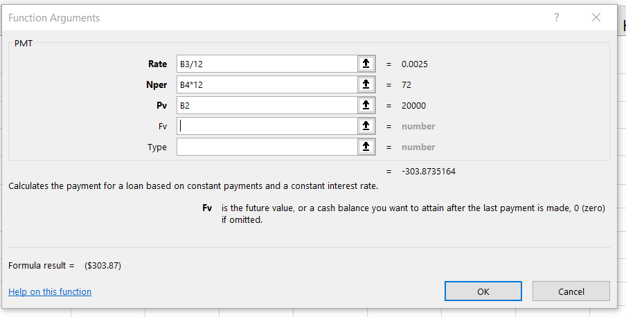
- You will now see the Rate, Nper, and Pv arguments defined for the function. (see Figure 2.31)
- Click the OK button at the bottom of the Function Arguments dialog box. The function will now be placed into the worksheet. Since we are not paying any lump sums of money at the end of the loan, there is no need to define the Fv argument. Also, we will assume that the monthly payments will be made at the end of each month. Therefore, there is no need to define the Type argument.
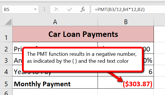
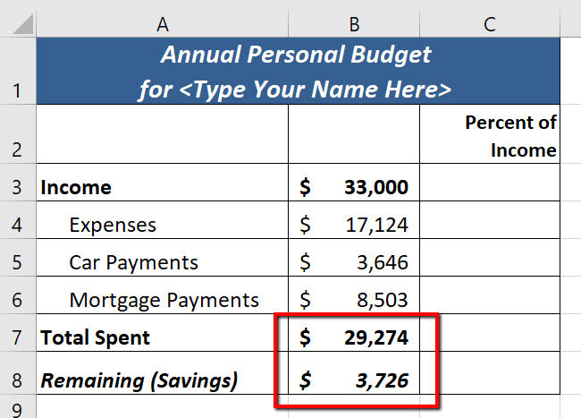
- Notice that the result of the formula in cell B5 is showing as a negative number (see Figure 2.32). To fix this, double-click on cell B5 and type a negative sign between the equal sign and the letters PMT in the formula (see Figure 2.33).
- The finished formula in cell B5 should be =-PMT(B3/12,B4*12,B2)
Figure 2.31 shows the completed Function Arguments dialog box for the PMT function. Notice that the dialog box shows the values for the Rate and Nper arguments. The Rate is divided by 12 to convert the annual interest rate to a monthly interest rate. The Nper argument is multiplied by 12 to convert the terms of the loan from years to months. Finally, the dialog box provides you with a definition for each argument. The definition appears when you click in the input box for the argument.
Keyboard Shortcuts
Insert Function
- Hold the SHIFT key while pressing the F3 key.
Function Arguments Dialog Box
- After the equal sign = and function name are typed into cell a location, hold down the CTRL key and press the letter A on your keyboard.
Integrity Check
Comparable Arguments for PMT Function
When using functions such as PMT, make sure the arguments are defined in comparable terms. For example, if you are calculating the monthly payments of a loan, make sure both the Rate and Nper argument are expressed in terms of months. The function will produce an erroneous result if one argument is expressed in years while the other is expressed in months.
The PMT Function when there is a down payment
In addition to calculating the loan payments for a car, the PMT function will be used in the Personal Budget workbook to calculate the mortgage payments for a home. The details for the mortgage payments are also found in the Loan Payments worksheet. Unlike the car loan, there is a down payment with the mortgage. A down payment on a mortgage is usually a percentage of the price of the home, which is paid up front and reduces the amount of the loan itself. The down payment amount and amount of the loan will both need to be calculated using formulas. While we did not use a down payment in the car loan example, it is fairly common to have a down payment when purchasing a car too.
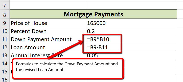
Write the formulas to calculate the Down Payment Amount and new Loan Amount by following these steps:
- Click cell B11.
- Write the formula =B9*B10. This will calculate 20% of the price of the house.
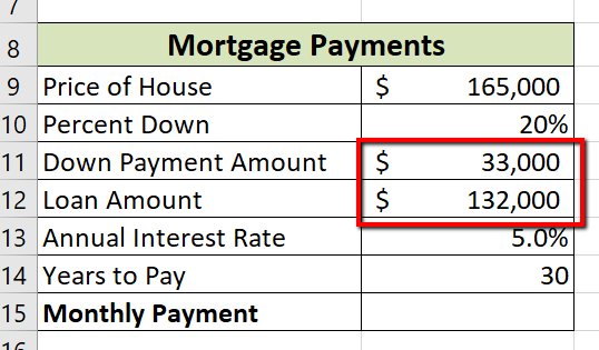
- Click cell B12. Write the formula =B9-B11. This will subtract the down payment amount from the price of the house (see Figure 2.34 for the Show Formulas View and Figure 2.35 for the formula results).
Now that we have the revised Loan Amount in cell B12, we can write the PMT function following the same process we did for the car loan.
- Click cell B15.
- Click the Formulas tab on the Ribbon.
- Click the Insert Function button to bring up the Insert Function dialog box.
- Type PMT in the search box and click Go.
- Double-click the PMT option in the “Select a function:” box. This will open the Function Arguments dialog box.
- Enter the following arguments (see Figure 2.36)
- Rate: B13/12 –> divide by 12 to convert the annual rate to a monthly one
- Nper: B14*12 –> multiply by 12 to convert the number of years into number of months
- Pv: B12 –> this is the cell with the actual loan amount, not the price of the house
- Click OK in the Function Arguments dialog box.
- Modify the formula in cell B15 to display the result as a positive number. Remember to type a negative sign between the equal sign and the letters PMT.
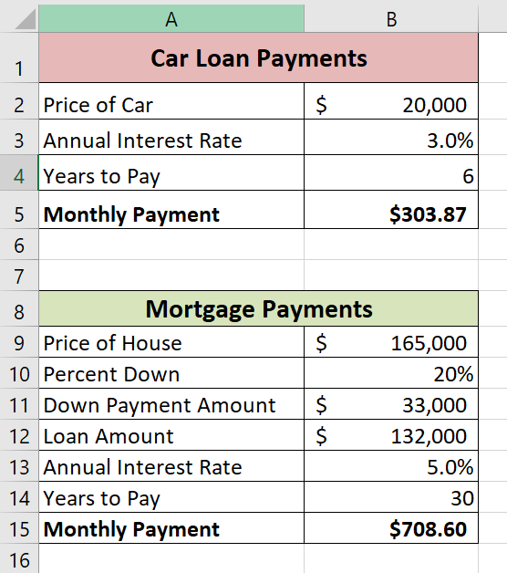
- Cell B15 should contain the function: =-PMT(B13/12,B14*12,B12) and the result should be $708.60 (see Figure 2.37).
Figure 2.36 shows how the the completed Function Arguments dialog box for the PMT function for the mortgage should appear before pressing the OK button.
Figure 2.37 shows the result of the PMT function for the mortgage. The monthly payments for this mortgage are $708.60. This monthly payment will be displayed in the Budget Summary worksheet.
Skill Refresher
PMT Function
- Type an equal sign =.
- Type the letters PMT followed by an open parenthesis, or double click the function name from the function list.
- Define the Rate argument with a cell location that contains the rate being charged by the lender for the loan or lease. If the interest rate given is an annual rate, divide it by 12 to convert it to a monthly rate.
- Define the Nper argument with a cell location that contains the amount of time to repay the loan or lease. If the amount of time is in years, multiply it by 12 to convert it to number of months.
- Define the Pv argument with a cell location that contains the principal of the loan or the price of the item being leased.
- Type a closing parenthesis ).
- Press the ENTER key.
- If the result needs to be shown as a positive number, add a negative sign between the equal sign and the letters PMT.
Linking Worksheets (Creating a Summary Worksheet)
So far we have used cell references in formulas and functions, which allow Excel to produce new outputs when the values in the cell references are changed. Cell references can also be used to display values or the outputs of formulas and functions in cell locations on other worksheets. This is how we will complete the Budget Summary worksheet using values from both the Budget Detail and Loan Payments worksheets.
Outputs from the formulas and functions that were entered into the Budget Detail will be displayed on the Budget Summary worksheet through the use of cell references.
- Switch to the Budget Summary worksheet and select cell B4. This cell needs to reference the Total Annual Spend (D12) from the Budget Detail worksheet.
- Type an =
- Click the Budget Detail worksheet tab.
- Click cell D12.
- Press the ENTER key on your keyboard.
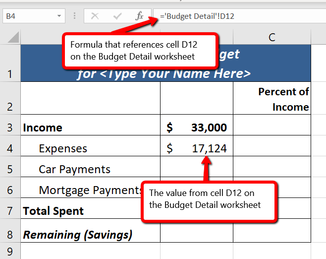
- The formula bar will display the formula =’Budget Detail’!D12 and the cell will display $17,124. (see Figure 2.38)
Figure 2.38 shows how the cell reference appears in the Budget Summary worksheet. Notice that the cell reference D12 is preceded by the Budget Detail worksheet name enclosed in apostrophes followed by an exclamation point (‘Budget Detail’!) This indicates that the value displayed in the cell is referencing a cell location in the Budget Detail worksheet.
We will use a similar process to enter in the annual car payments and mortgage payments from the Loan Payments worksheet. The payments on the Loan Payments worksheet are monthly payments though, so we will need to multiply each one by 12 to get the annual amount to display in the Budget Summary worksheet.
- Click on cell B5. This cell needs to contain a formula that references the monthly car payment cell (B5) on the Loan Payments worksheet and multiplies by 12.
- Type an =
- Click the Loan Payments worksheet tab.
- Click cell B5 on the Loan Payments worksheet.
- The formula bar will display the formula =’Loan Payments’!B5
- Type an asterisk * for multiplication.
- Type the number 12. The formula in the formula bar should read: =’Loan Payments’!B5*12
- Press the ENTER key on your keyboard.
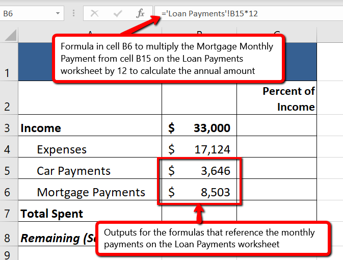
- Click on cell B6. This cell needs to contain a formula that references the monthly mortgage payment cell (B15) on the Loan Payments worksheet and multiplies by 12.
- Type an =
- Click the Loan Payments worksheet tab.
- Click cell B15 on the Loan Payments worksheet.
- The formula bar will display the formula =’Loan Payments’!B15
- Type an asterisk * for multiplication.
- Type the number 12. The formula in the formula bar should read: =’Loan Payments’!B15*12
- Press the ENTER key on your keyboard.
Figure 2.39 shows the results of creating formulas that reference cell locations in the Loan Payments worksheet.
We can now add other formulas and functions to the Budget Summary worksheet that can calculate the difference between the total spend dollars vs. the total net income in cell B3. The following steps explain how this is accomplished:
- Click cell B7 in the Budget Summary worksheet.
- Type an equal sign =.
- Type the function name SUM followed by an open parenthesis (.
- Highlight the range B4:B6.
- Type a closing parenthesis ) and press the ENTER key on your keyboard or simply press the ENTER key to close the function. The total for all annual expenses now appears on the worksheet.
- Click cell B8 on the Budget Summary worksheet. You will enter a formula to calculate Remaining (Savings) amount in this cell.
- Type an equal sign =.
- Click cell B3.
- Type a minus sign − and then click cell B7.
- Press the ENTER key on your keyboard. This formula produces a positive number, indicating our income is greater than our total expenses.
Figure 2.40 shows the results of the formulas that were added to the Budget Summary worksheet. Overall, having your income exceed your total expenses is a good thing because it allows you to save money for future spending needs or unexpected events.
We can now add a few formulas that calculate both the spending rate and the savings rate as a percentage of net income. These formulas require the use of absolute references, which we covered earlier in this chapter. The following steps explain how to add these formulas:
- Click cell C7 in the Budget Summary worksheet.
- Type an equal sign =.
- Click cell B7.
- Type a forward slash / for division and then click B3.
- Press the F4 key on your keyboard. This adds an absolute reference to cell B3.
- Press the ENTER key. The result of the formula shows that total expenses consume 89% of our net income.
- Click cell C7.
- Place the mouse pointer over the Auto Fill Handle.
- When the mouse pointer turns to a black plus sign, left click and drag down to cell C8. This copies and pastes the formula into cell C8.
- Compare your worksheets with Figures 2.41a-c below. Make any necessary changes before moving on to the next section.
- Save the CH2 Personal Budget file.
Figure 2.41a shows the completed Budget Summary worksheet
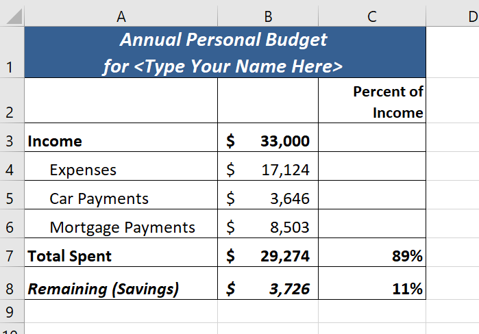
Figure 2.41b shows the completed Budget Detail worksheet
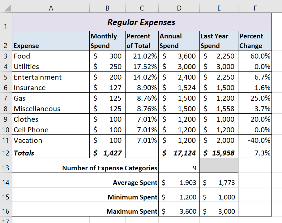
Figure 2.41c shows the completed Loan Payments worksheet
Key Takeaways
- The PMT function can be used to calculate the monthly mortgage payments for a house or the monthly lease payments for a car.
- When using the PMT function, each argument must be separated by a comma.
- To calculate the monthly payment for a loan using the PMT function, the Rate and Nper arguments must be defined in terms of months. The Rate should be divided by 12 to convert it from an annual rate to a monthly rate. The Nper should be multiplied by 12 to convert the term of the loan from years to months.
- The PMT function produces a negative output if the Pv argument is not preceded by a minus sign. For the purposes of this textbook, a minus sign will be entered before the PV argument in the PMT dialog box.
Attribution
Adapted by Mary Schatz from How to Use Microsoft Excel: The Careers in Practice Series, adapted by The Saylor Foundation without attribution as requested by the work’s original creator or licensee, and licensed under CC BY-NC-SA 3.0.