5.2: Intermediate Table Skills

Learning Objectives

• Sort table data.
• Custom Sort table data.
• Apply Custom List sort options.
• Filter table data using criteria filters.
• Use the Advanced Filter option to filter table data.
• Analyze data with PivotTables & Subtotals.

INTERMEDIATE TABLE SKILLS

SORT, FILTER, AND ANALYZE DATA WITH PIVOT TABLES & SUBTOTALS

SORTING

Sorting is one of the most common tools for data management. By arranging data sequentially the information becomes more meaningful. Arranging records in a specific sequence is called sorting. If you sort by one column this is considered a single sort. If you need to sort by more than one column, this is considered a custom sort.

The field or fields you select to sort are called sort keys. In Excel, you can sort your table by ascending or descending order. Data in ascending order appears lowest to highest, earliest to most recent, or alphabetically from A to Z. Data in descending order in arranged by highest to lowest, most recent to earliest, or alphabetically from Z to A.

Excel will sort a range of data that is not in a table. However, when working with large sets of information it is wise to make the data a table for integrity. Excel locks the row of information creating a record, thus when sorted, the record remains intact, just reorganized. For example, when you sort the table by last name, all of the records in each row move together. It is always a good idea to save a copy of your worksheet before applying sorts.

There are multiple places you can find and use sorting tools:

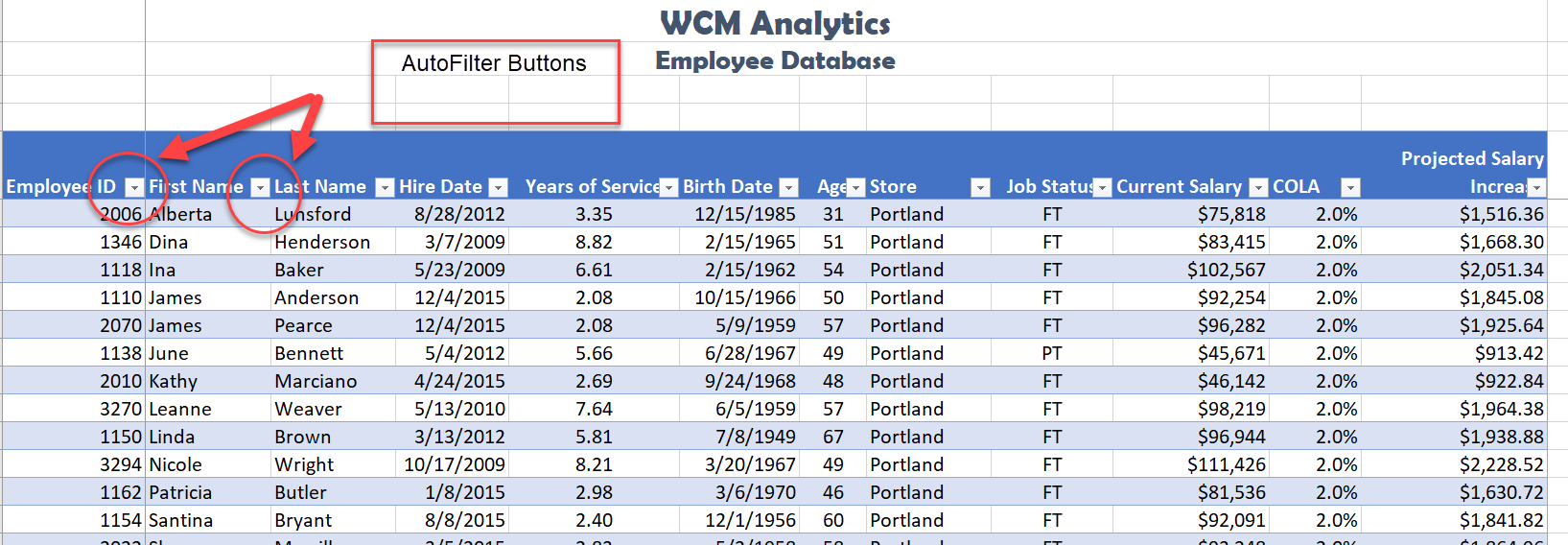
• When you first create a table, Excel automatically enables AutoFilter buttons; a tool used to sort, query, and filter the records in a table. The filter buttons appear to the right of the column headings. When you click the filter button sorting options appear on the menu options.

Figure 5.23 AutoFilter Buttons

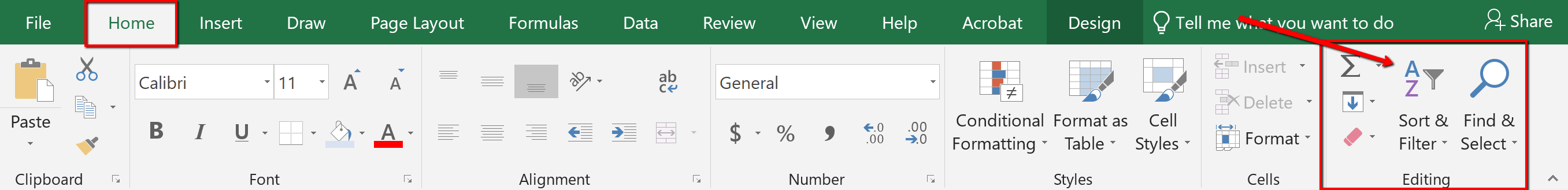
• From the Home tab, in the Editing group, click the ‘Sort & Filter’ button, and then click one of the sorting options on the Sort & Filter menu.

Figure 5.24 Sort and Filter Menu

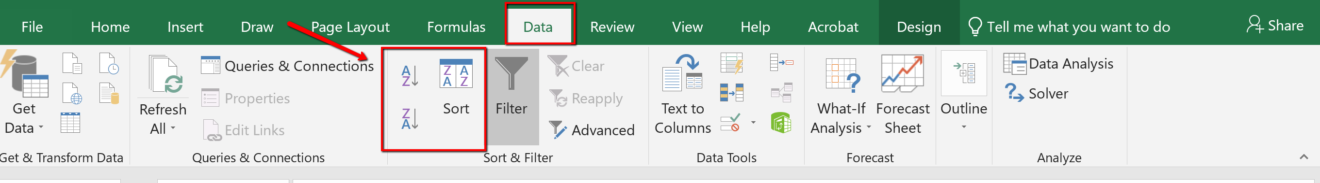
• From the Data tab, use the ‘Sort A to Z’ or ‘Sort Z to A’ buttons or for multiple levels select the Sort button to open the Custom Sort dialogue.

Figure 5.25 Data Tab Sort options

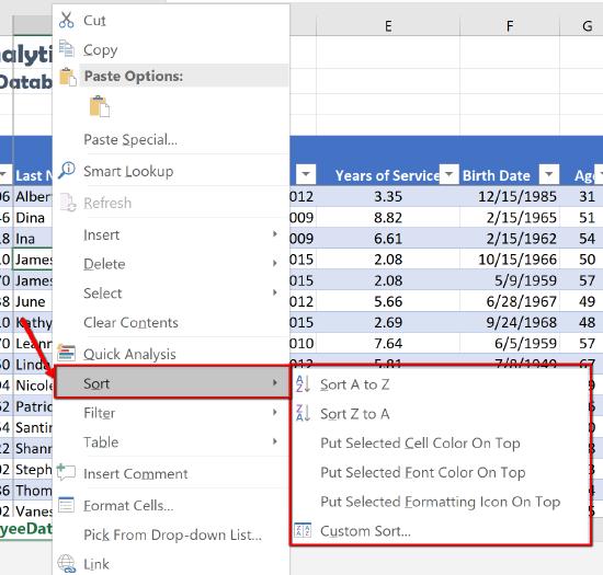
• Right-click anywhere in a table and then point to Sort on the shortcut menu to display the Sort sub-menu.

Figure 5.26 Right-Click Menu

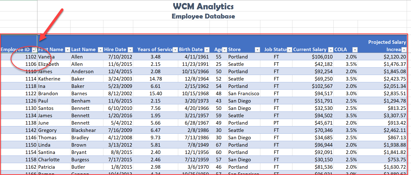
Complete a single level sort by following the steps:

1. In the EmployeeID heading, click the filter button.
2. Choose to Sort Smallest to Largest.

      Mac Users: Click the A-Z Ascending button

Notice Excel arranges in chronological order all the employee data based on the EmployeeID number, however keeping each record together. You will also notice the filter button now displays an up arrow denoting an ascending sort.

Figure 5.27 EmployeeID Sort

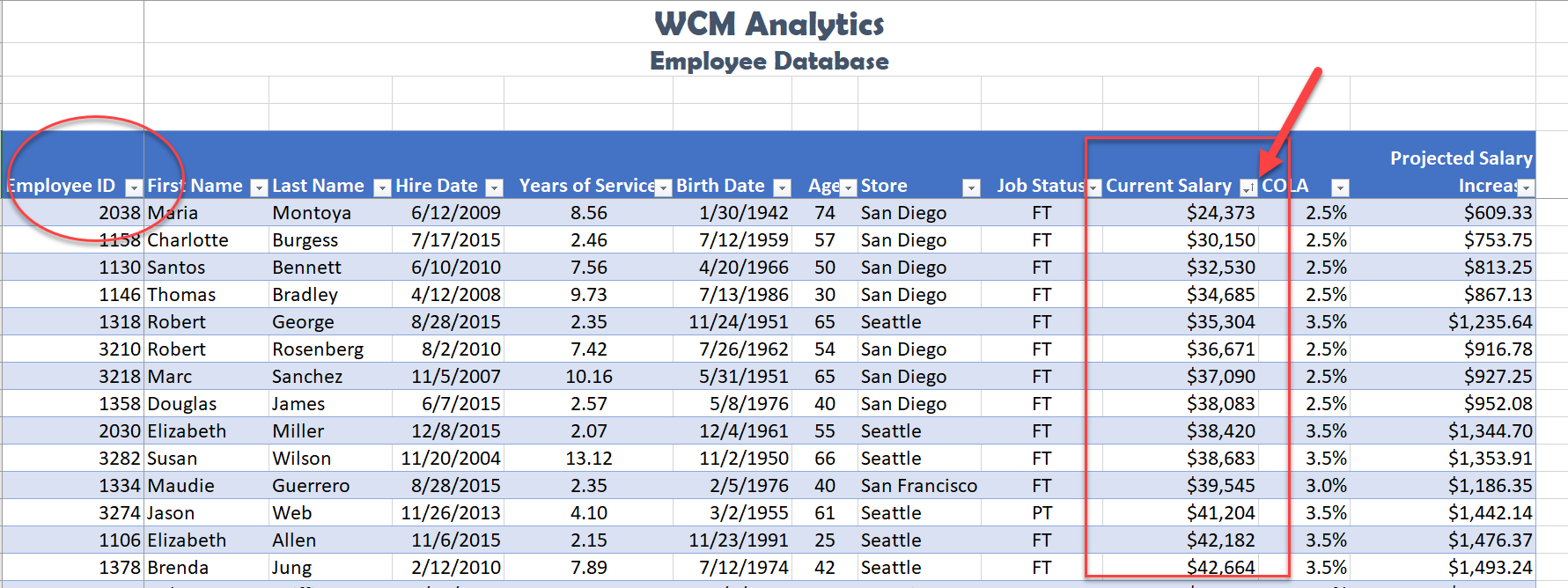
The following steps will sort the records in descending order by Current Salary using the ‘Sort Largest to Smallest’ option form the filter button.

1. Click the filter button located in the Current Salary heading.
2. Choose Sort Largest to Smallest option from the menu. 

      Mac Users: click the “Descending” button

Notice the original sort has been overridden, and the information is now organized based on the largest Current Salary. You will see the small arrow on the EmployeeID filter is gone, and an arrow pointing down for Descending Order is visible on the Current Salary filter button.

Figure 5.28 Current Salary Sort

Skill Refresher

Sort a Column

1. Click on the filter Click arrow to the right of the header in the column you want to sort.
2. Click on the choice AZ↑ or ZA↓ to sort your data by that column.

CUSTOM SORT

When you need to sort by more than one level, you must use the Custom Sort option. Complete the following steps to organize the data by Store, Last Name, Current Salary, all in Ascending Order (A-Z).

1. Select the Data tab, and click the Sort button. Notice the last column sorted by is listed. Change the column heading name by dropping down the Sort by menu and select Store.
2. Click Add Level.

     Mac Users: click the + symbol

3. Click the down arrow in the Then by section, and choose the column heading names as shown below in Figure 5.29. Note to click Add Level to add the next column heading. The order you select the headings will determine how the table information is sorted.

Figure 5.29 Sort Dialogue Box

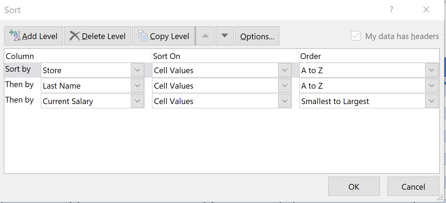
4. Once you select to Sort by column headings, choose the Order by selecting to sort in ascending order (A-Z) for the Store and Last name fields, and Smallest to Largest, for the Current Salary field.
5. Click OK.

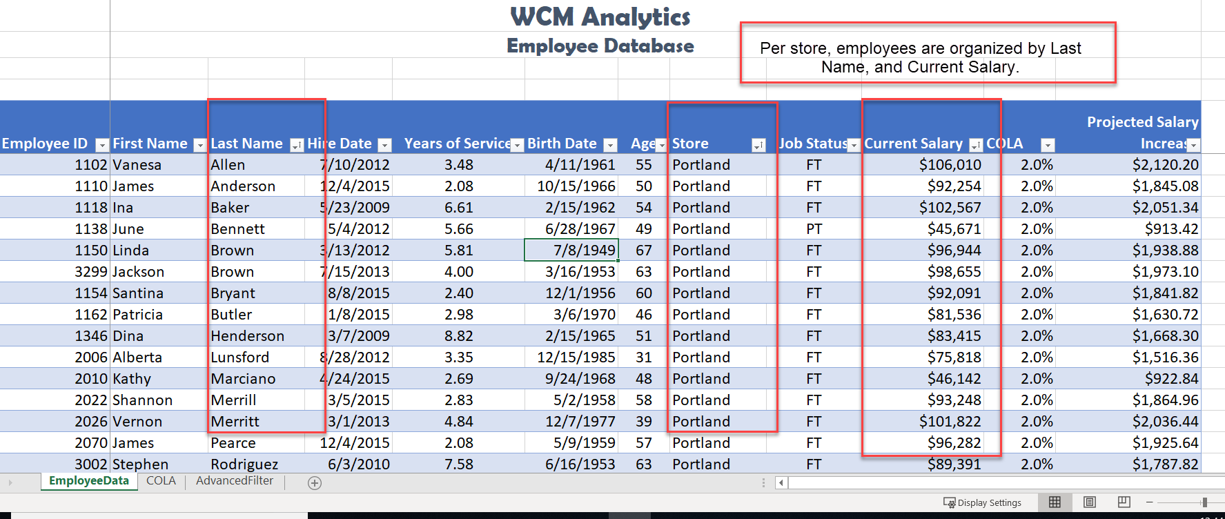
Notice the information is now sorted by three levels, per Store , each employee is organized by Last Name , and Current Salary in ascending order (smallest to largest). Each of the filter buttons indicates the sort with the up arrow.

Figure 5.30 Custom Sort Visual

Skill Refresher

Custom Sort (Multiple Level Sort)

1. Select the Data tab, and click the Sort button.
2. Choose Add Level.
3. Click the down arrow in the Column field and choose the column heading to sort by.
4. Repeat the above steps to add another level and select the next column heading to sort by.
5. The order you select the headings will determine how the table information is sorted.

CUSTOM LIST SORT

When sorting you can create custom lists that allow sorting by characteristics that do not sort alphabetically. Example, text items such as high, medium, and low—or S, M, L, XL. Dates commonly require custom lists so you can vary in the way data is sorted by days of the week or months of the year.

In our case, we want to create a custom list that sorts our stores, which is not, in ascending or descending order. The human resources office likes to order the stores based on the location size. The company headquarters is in Seattle and employs the most people. The next biggest location is San Diego etc. Follow the below steps to create a custom list ordering the stores as shown below:

Seattle

San Diego

Portland

San Francisco

 

Mac Users: The steps to create a custom sort list are different for Excel for Mac. Please skip the below steps and follow the alternate steps below Figure 5.34.

Follow the below steps to create a custom list ordering:

1. While clicked in the table, choose the Data tab and click the Sort button.
2. In the Sort by row, click the drop-down menu in the Order Column for the Store heading. Choose Custom List.

Figure 5.31 Custom List Dialogue Box

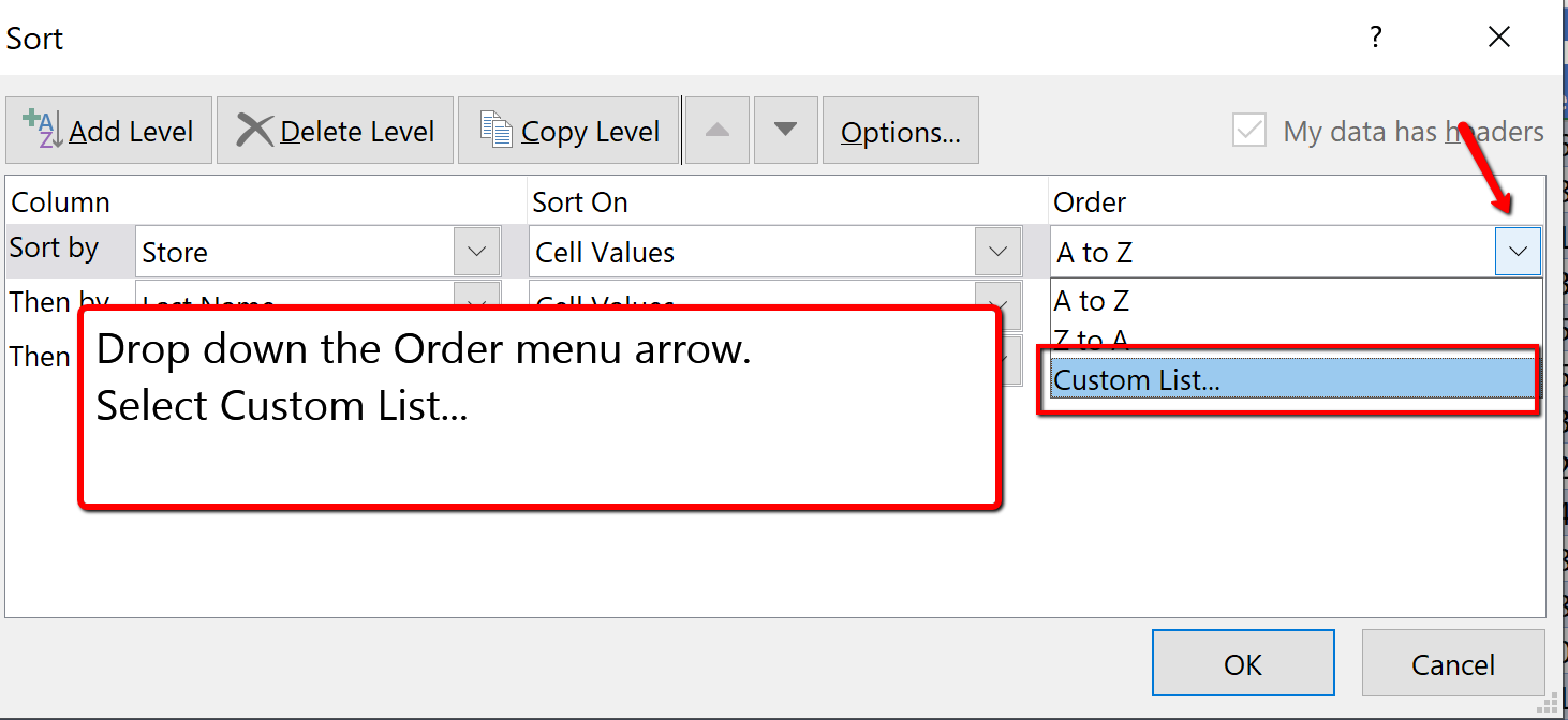
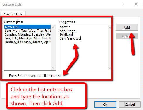
3. Click in the List entries: box and type Seattle, and press enter. Type the remainder of the locations shown in Figure 5.32, pressing enter after each store location typed. Once all locations are entered, click Add. Then choose Ok.

Figure 5.32 Custom List Entries dialogue box

4. You will see the Order of the Store sort update. Click OK to close the Sort dialogue box.

Figure 5.33 Sort_Dialogue Box Custom List Order

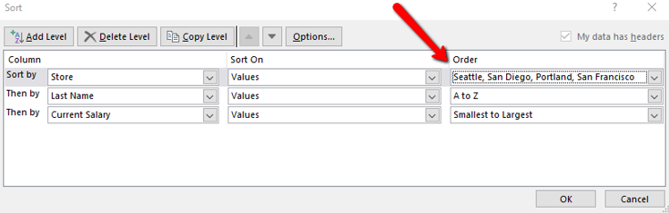
The custom sort is applied and the table is now sorted by Store, using the custom order, then the Last Name of the employee and then by the Current Salary column.

Figure 5.34 Custom List Sort Visual

Mac Users alternate steps for creating a custom sort list:

1. Click the Excel menu option and choose Preferences
2. Click on the Custom List button
3. Type the list of cities in the “List entries” box as shown in Figure 5.32 above then click the Add button and close the Custom List dialog box
4. Click anywhere in the table, and then click the Data tab and click the Sort button
5. Click the drop-down menu in the Order Column for the Store heading. Choose Custom List
6. Click on the custom list of cities that you just created and then click the OK button twice
7. The custom sort is applied and the table is now sorted by Store, using the custom order, then the Last Name of the employee and then by the Current Salary column. See Figure 5.34 above.

Skill Refresher

Custom List Sort

1. Select the Data tab, and click the Sort button.
2. Click the drop-down menu in the Order Column of the field needing a custom list created.
3. Choose Custom List.
4. Click in the List entries box and type the custom list desired.
5. Then click Add.
6. Click Ok.

FILTER DATA

If your worksheet contains a lot of data, it can be difficult to find information quickly. Applying Filters is an efficient and effective way to only show the information needed. Typically when filtering you are searching the data for specific information. Generally speaking, you are searching the data based on a question, or in other words, querying the data, and returning only the information that satisfies the question. The process of filtering records based on one or more filter criteria is called a query. Filtering data hides the rows whose values do not match the search criteria. The information that does not display is not deleted, it is just hidden, and will be redisplayed by removing the filter or applying a new filter.

Like sorting, Filter options are located in the filter button alongside each field name. By clicking the filter button, you can choose which values in that field to display, hiding the rows or records that do not match that value. The filter lets you choose to display only those records that meet specified criteria such as color, number, or text. In this situation, criteria is defined as; a logical rule by which data is tested and chosen.

For example, you can filter the table to display a specific name or item by typing it in a Search box. The name you selected acts as the criterion for filtering the table, which results in Excel displaying only those records that match the criterion. The selected checkboxes indicate which items will appear in the table. By default, all of the items are selected. If you deselect an item from the filter menu, it is removed from the filter criterion. Excel will not display any record that contains the unchecked item. As with the previous sort techniques, you can include more than one column when you filter by clicking a second filter button and making choices. After you filter data, you can copy, find, edit, format, chart, or print the filtered data without rearranging or moving it.

Figure 5.35 Filter Search Menu

Complete the following steps and filter data according to each query.

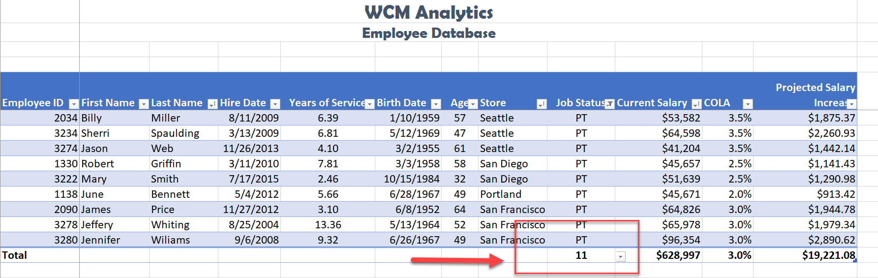
How many employees are at a Part-Time (PT) status?

1. Click the filter button on the Job Status column heading.
2. Click Select All, to deselect options.
3. Click the PT box to only display the part-time employees.
4. From the total row, in cell I108, choose the Count function count the number of employees at a PT status.

The answer to the question is there are currently are 11 employees at a PT time status. The total row will display the part-time total current salaries, and what the projected salary increase for part-time help will be after COLA adjustments.

Figure 5.36 PT Filter Visual

USING CRITERIA FILTERS

The filters created are limited to selecting records for fields matching a specific value or set of values. For more general criteria, you can use criteria filters, which are expression involving dates and times, numeric values, and text strings. Excel will identify what criteria filter to display based on the information in the column. For example, you can filter the employee data to show only those employees hired within a specific date range. Notice the criteria filter changes to Date Filters. If we were looking at the Current Salary column, the filter would be a Numbers Filter.

Using criteria filters, follow the below steps to search for employees who have been with the company for a specific time period.

Identify employees who have been with the company between 2013-2016.

1. While clicked in the table, clear any sort or filter applied by clicking the Data tab. In the Sort & Filter group choose the Clear button.
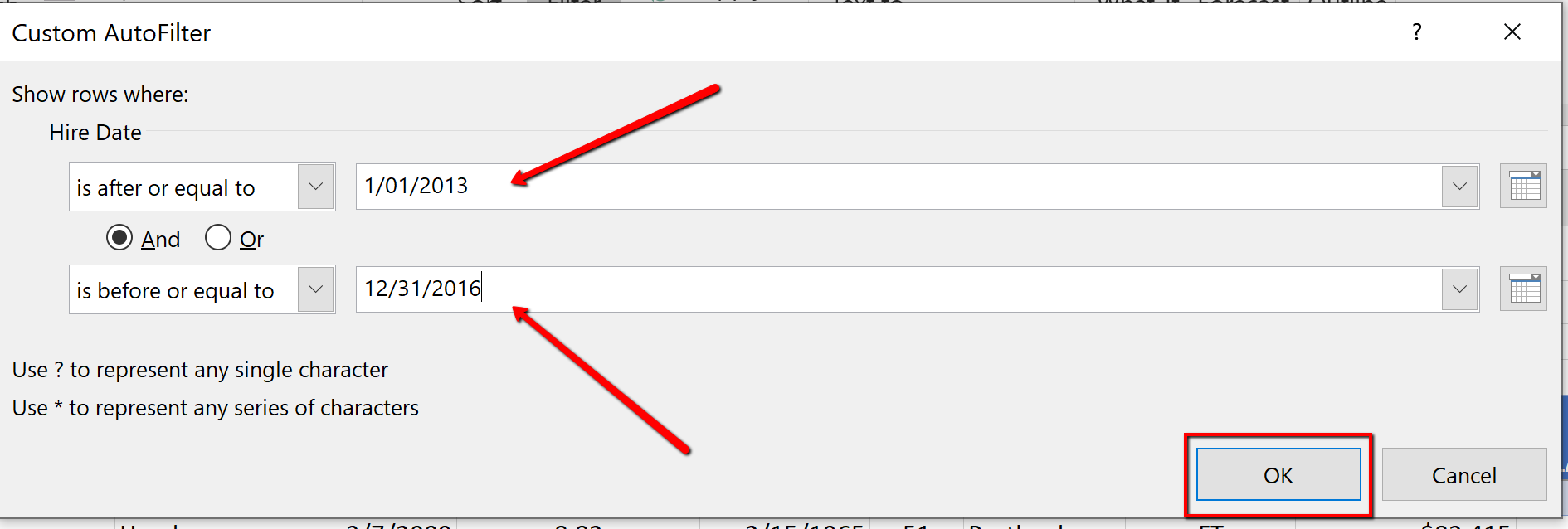
2. Click the Filter button in the Hire Date column. Select Date Filters, and choose the Between criteria.

      Mac Users: uncheck the Select All checkbox before choosing the Between option.

Figure 5.37 Date Filter Menu

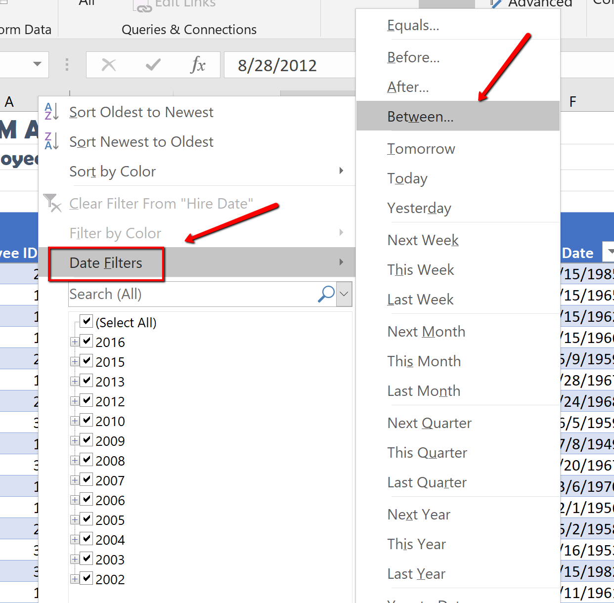
3. Search for employees with a hire date between 2013, and 2016. In the “is after or equal to” section type 1/01/2013, and typing in the “is before or equal to” section type 12/31/2016. Then click OK.

     Mac Users: Excel for Mac sections simply say “After” and “Before”

Figure 5.38 Date Filter Between Dialogue Box

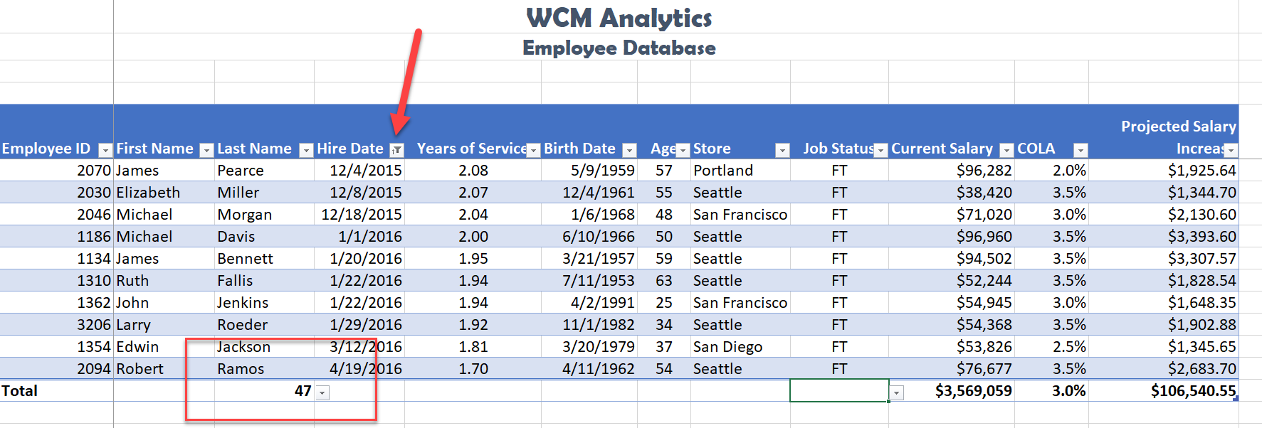
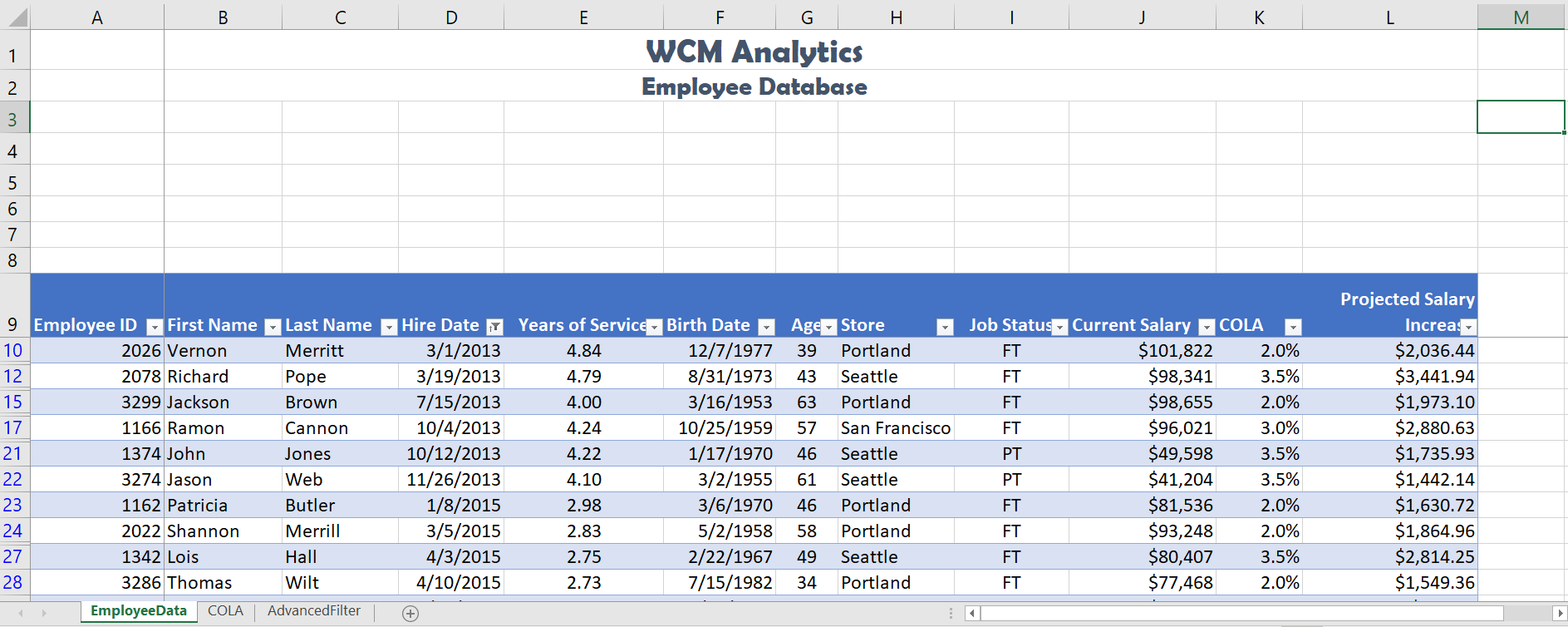
4. Sort the filtered table from Oldest to Newest by Date Hired.
5. In the total row section, count the last name names of the employees by applying the count function in cell B108.
6. In the total row, select cell I108, and choose None to turn off the count function in the Job Status Column.

Notice the table total row show 47 employees hired between the specified dates. These employees will be evaluated for a COLA adjustment.

Notice the filter button displays a filter symbol and an up arrow indicating the column is filtered and sorted in ascending order.

Figure 5.39 Date Filter and Sort

SLICERS

Another way to filter an Excel table is with slicers. Slicers, generally speaking, are visual filter buttons you can click to filter the table data. Slicers show the current filtered category, which makes it easy to understand what exactly is displayed. For example, a slicer for the Store field would have buttons for the Seattle, San Diego, Portland, and San Francisco locations.

When slicer buttons are selected, the data is filtered to show only those records that match the criteria. Multiple buttons can be selected at the same time, and a table can have multiple slicers, each linked to a different field. When multiple slicers are used, Excel uses the AND logical operator so filtered records must meet all of the criteria indicated in the slicer. When selecting multiple buttons in a Slicer, use the shift key to select adjacent field names. If the field names are not adjacent, use the non-adjacent selection method, pressing the CTL button, and selecting the field names needed.

Follow the below steps to filter the table using visual Slicer buttons.

1. Click in the table area. From the Data tab, choose Clear to remove the current sort and filter applied to the data.
2. To make room for the Slicer buttons at the top of the table, we will add 4 rows between the title and the table area. Right-click cell A3. Choose Insert. Select Entire Row. Repeat these steps until the table heading starts in row A9.

      Mac users should hold down CTRL key and click cell A3. Then repeat until the table heading starts in row A9.

Figure 5.40 Added Rows

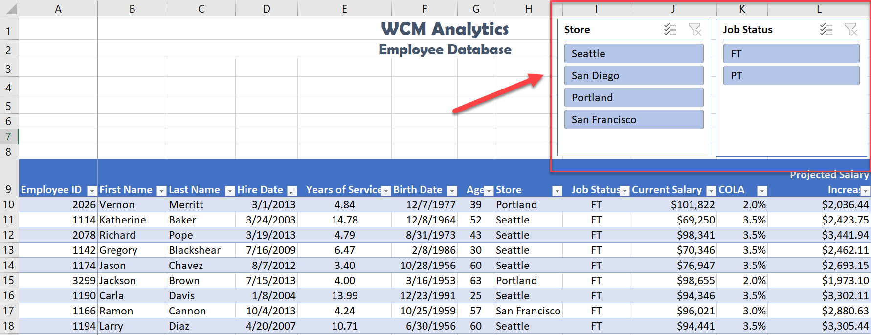
3. Click back into the table area. Choose the Insert tab. Click Slicer. When the Insert Slicers dialogue box opens, click the Store and Job Status field names to display as slicers. Click OK.

Figure 5.41 Slicer Dialogue Box

 

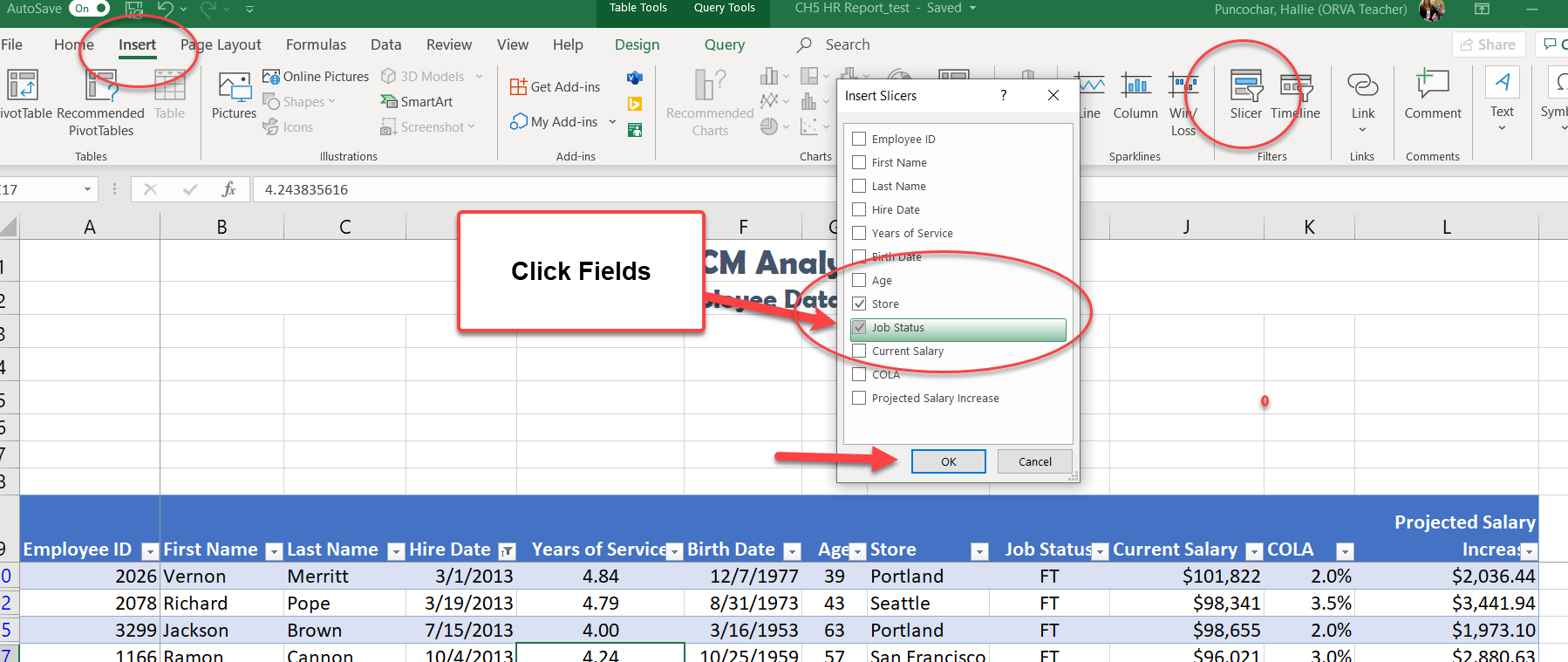
4. Move, and re-size the Slicer boxes to fit in the approximate area of I1:J8 and K1:L8. Make sure the buttons remain visible. Below is a visual example.

Figure 5.42 Slicer Layout Example

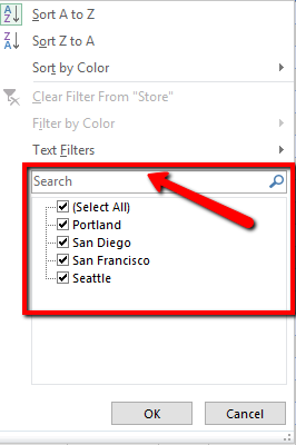
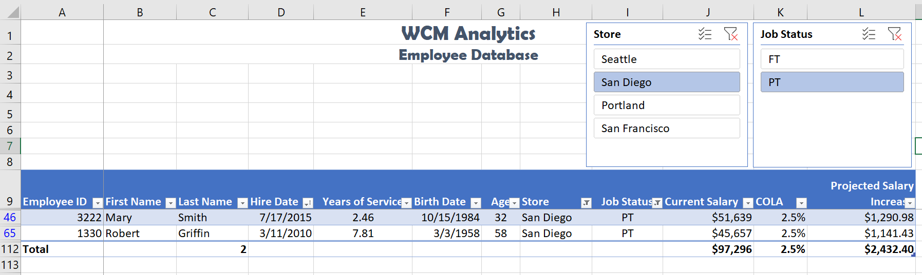
5. From the Store slicer, click the San Diego button. Notice the data filters to only show the data for San Diego.
6. From the Job Status slicer click PT. Notice the data filters to only show the data for PT employees in San Diego.

Figure 5.43 Slicer Solution

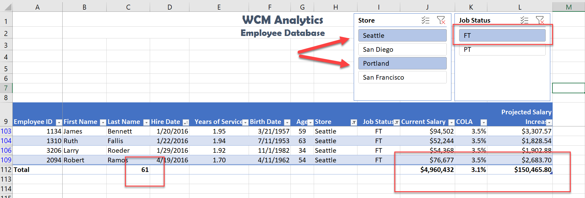
7. Return to the Store slicer and choose Seattle and Portland. Note the non-adjacent selection method is needed. Select Seattle first, then press and hold the Ctrl button on the keyboard, and then select Portland.

      Mac Users: hold down the Command key not the Ctrl key before you click on Portland.

8. Change the Job Status slicer selection to FT.

The table results show there are 61 FT employees in Seattle and Portland. The Projected Salary Increase after the COLA adjustment for the Northwest region is $150,465.80.

Figure 5.44 Non-Adjacent Slicer Solution

ADVANCED FILTERS

Filter buttons are limited to combining fields using advanced logic or complex criteria. If the data you want to filter requires complex criteria, you can use the Advanced Filter dialog box. The Advanced Filter works differently from the Filter command in several important ways:

• It displays the Advanced Filter dialog box instead of the AutoFilter menu.
• You type the advanced criteria in a separate criteria range in a worksheet and above the range of cells or table that you want to filter. Excel uses the separate criteria range in the Advanced Filter dialog box as the source for the advanced criteria.

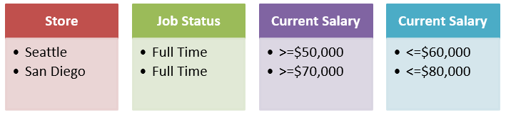
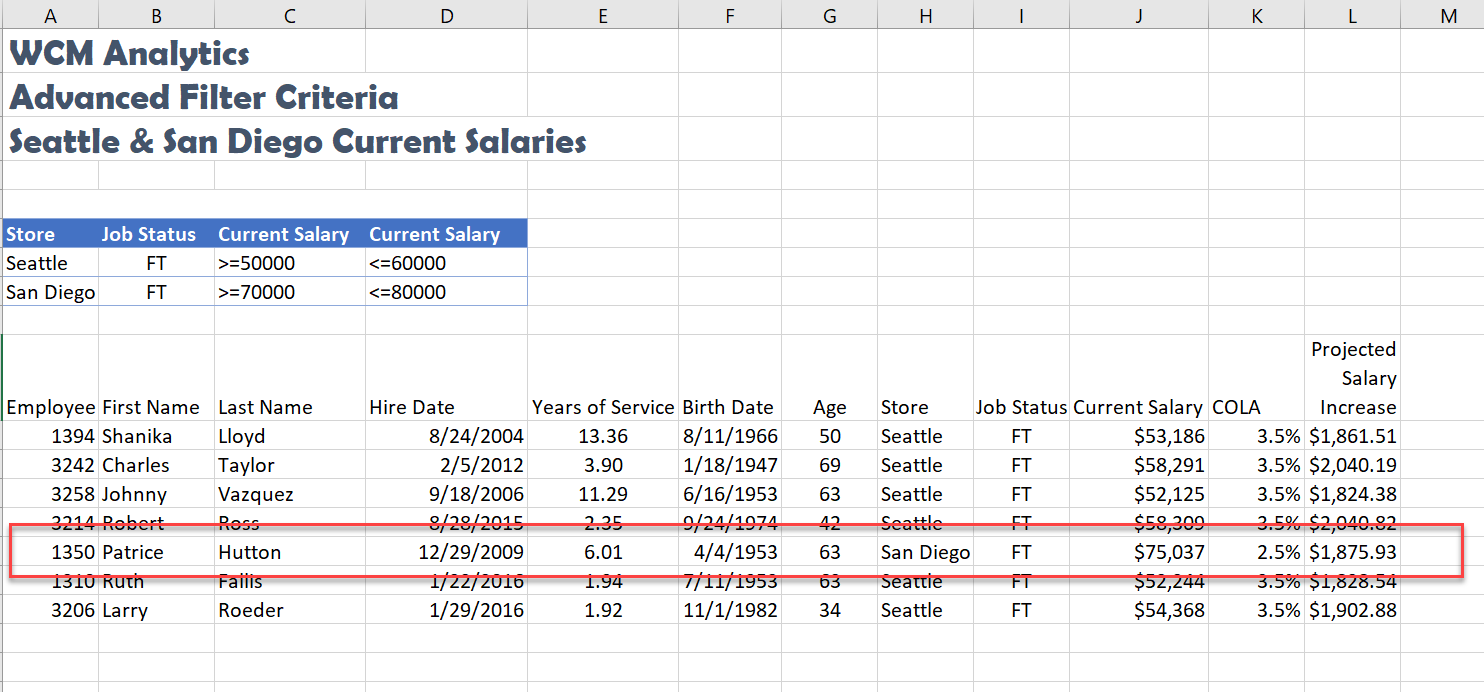
For example, you searched records for employees in the Seattle and San Diego offices AND for employees working at full-time bases, AND have a base salary between the below Salary Ranges:

Figure 5.45 Advanced Filter Criteria

To run the above complex criteria mentioned above follow the below steps:

1. From the EmployeeData sheet, click in the table, then select the Data tab and clear the current filters by selecting the Clear button.
2. Select the Table Tools Design tab and turn off the Total Row.
   Mac Users: just click the Table tab and turn off the Total Row
3. Select the Advanced Filter sheet. Click cell A10. The criteria mentioned in the above example has already been entered for this advanced filter exercise. Next, you will use an advanced filter to copy the records that match these criteria.
4. From the Data tab, click the Advanced button. The Advanced Filter dialog box opens.
5. Click the Copy to another location option button to copy matching records from the data range.
6. Click in the List range box to make it active, and then navigate to the EmployeesData sheet, click cell A9, and then press and hold the CTRL and SHIFT and SPACEBAR to select the entire table. In the List range box, you will see Employee_DB[#All] in the list range box.
   Mac Users: The keyboard shortcut of “CTRL, SHIFT, SPACEBAR” does not work in Exel for Mac. You should click in Cell A9, scroll down to the end of the data, hold down the Shift key and click in Cell L112 to select the entire table
7. Click, or press the tab key, to move to the Criteria Range box.
8. From the Advanced Filter sheet, select A6:D8. You will see ‘Advanced Filter’!Criteria populate in the criteria range box.
9. Click, or press the tab key, to move to the Copy to box, and then click cell A10 to specify the location for inserting the copied records. You will see ‘Advanced Filter’!$A$10 in the Copy to criteria range box.

Figure 5.46 Advanced Filter Dialogue Box

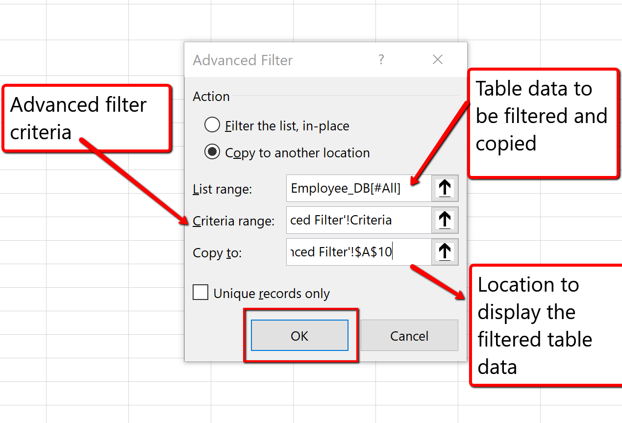
10. Click OK to copy the records that match the advanced filter criteria. Save your work.

The advanced search results list 7 employees that meet the criteria. Of these 7 employees, only 1 full-time employee in San Diego has a current salary between $70,000 and $80,000 dollars, and 6 full-time Seattle employees have a current salary between $50,000 and $60,000 dollars.

Figure 5.47 Advanced Filter Results

INSERT TABLE

 

Let’s review another away to turn a range of data into a table.

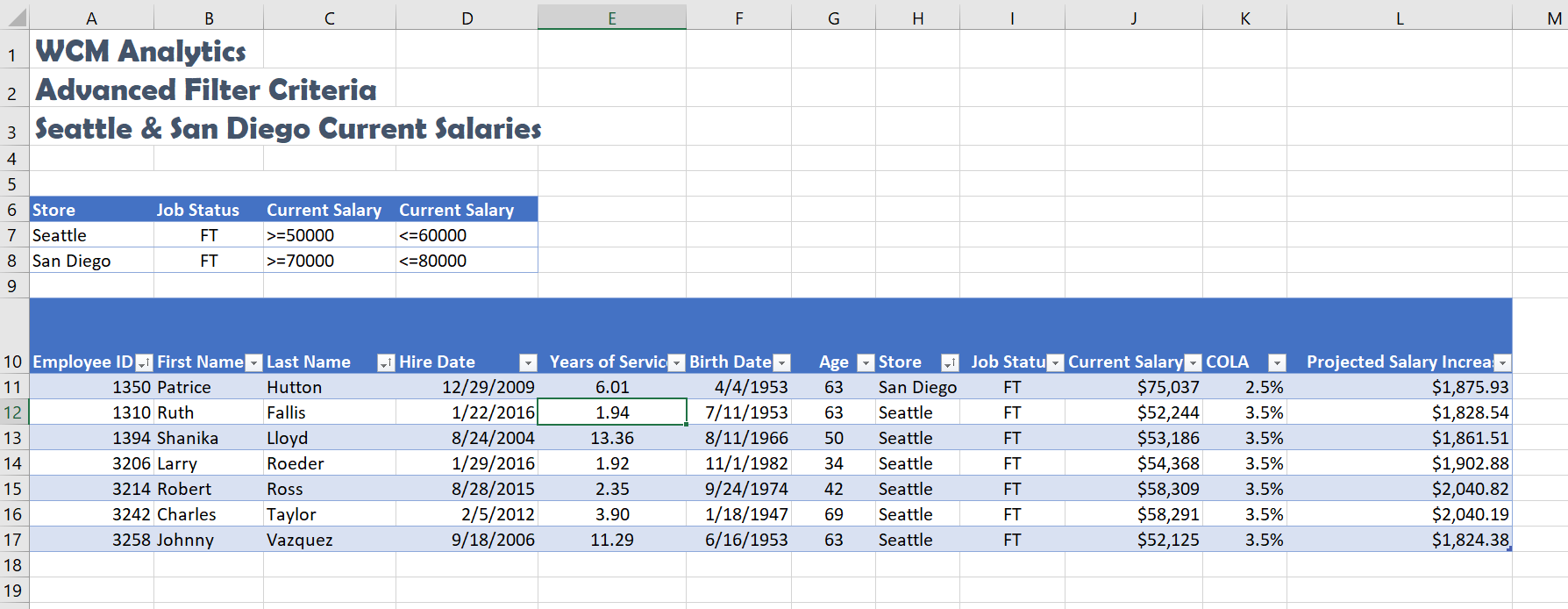
1. Select the Advanced Filter sheet, and click cell A10.
2. From the Insert tab, choose Table.
3. The Create Table dialogue box will appear.
4. Make sure “My table has headers” is selected so Excel recognizes the column headings.
5. Click OK. Excel turns our advance search data into a table.
6. Sort the table in ascending order (A-Z), by Store, and Employee ID, then Last Name. Hint: Click the Data tab, Click the Sort button, add levels for the three fields.
7. Autofit the column widths and row height to make sure the heading row is visible.
8. Save your work.

Excel turns the information into a table and sorts accordingly:

Figure 5.48 Advanced Filter Table

ANALYZING WORKSHEET DATA

INTRODUCTION TO PIVOT TABLES

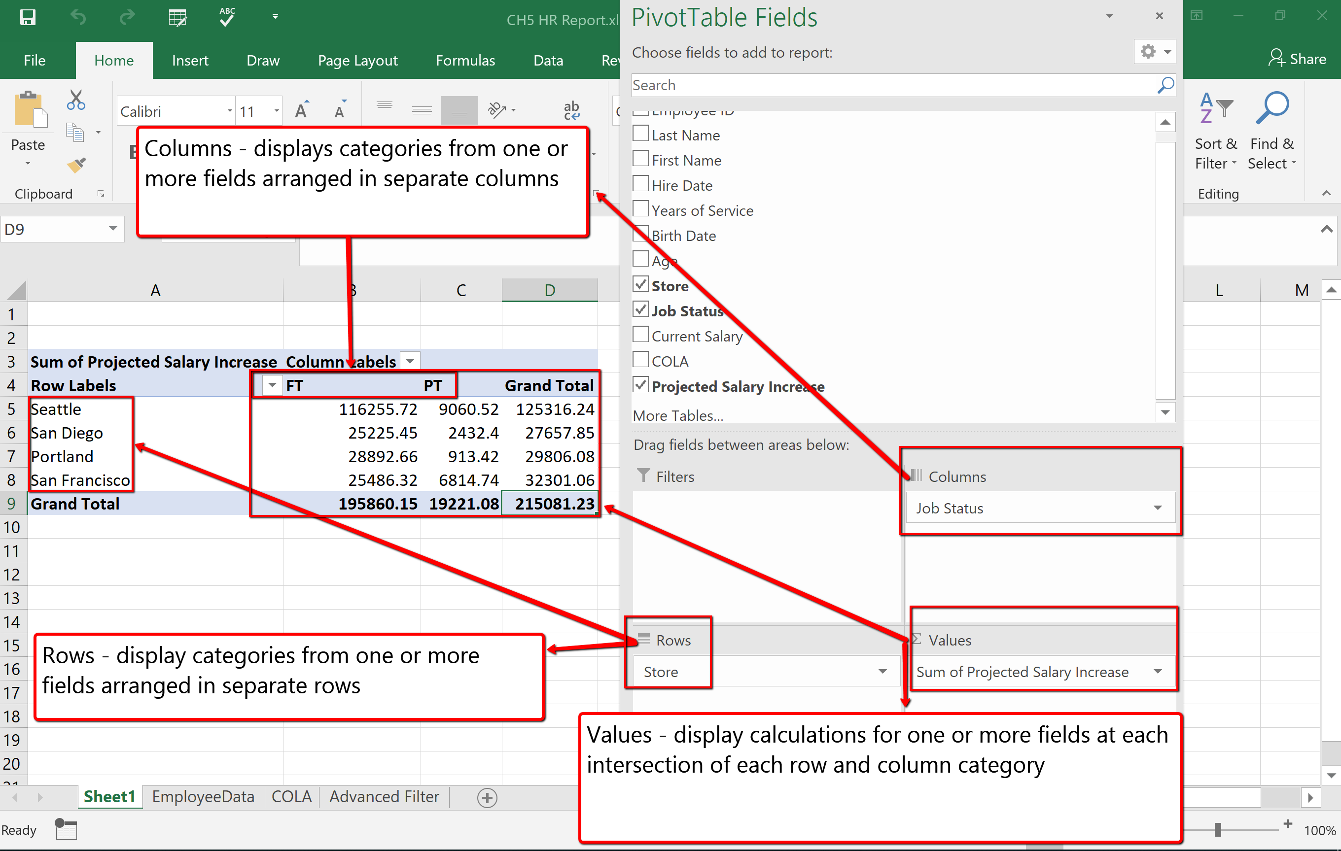
Another way to analyze table information is with PivotTables. A PivotTable is a powerful tool that calculates, summarizes, and analyzes table data to compare, patterns, and trends. PivotTables are inserted directly from a table, linking the table data. Generally speaking, when you pivot on the table data you are reorganizing the table information to reveal different levels of detail that allow you to analyze specific subgroups of information and summarize data quickly and easily without having to change the structure or layout of the original table area.

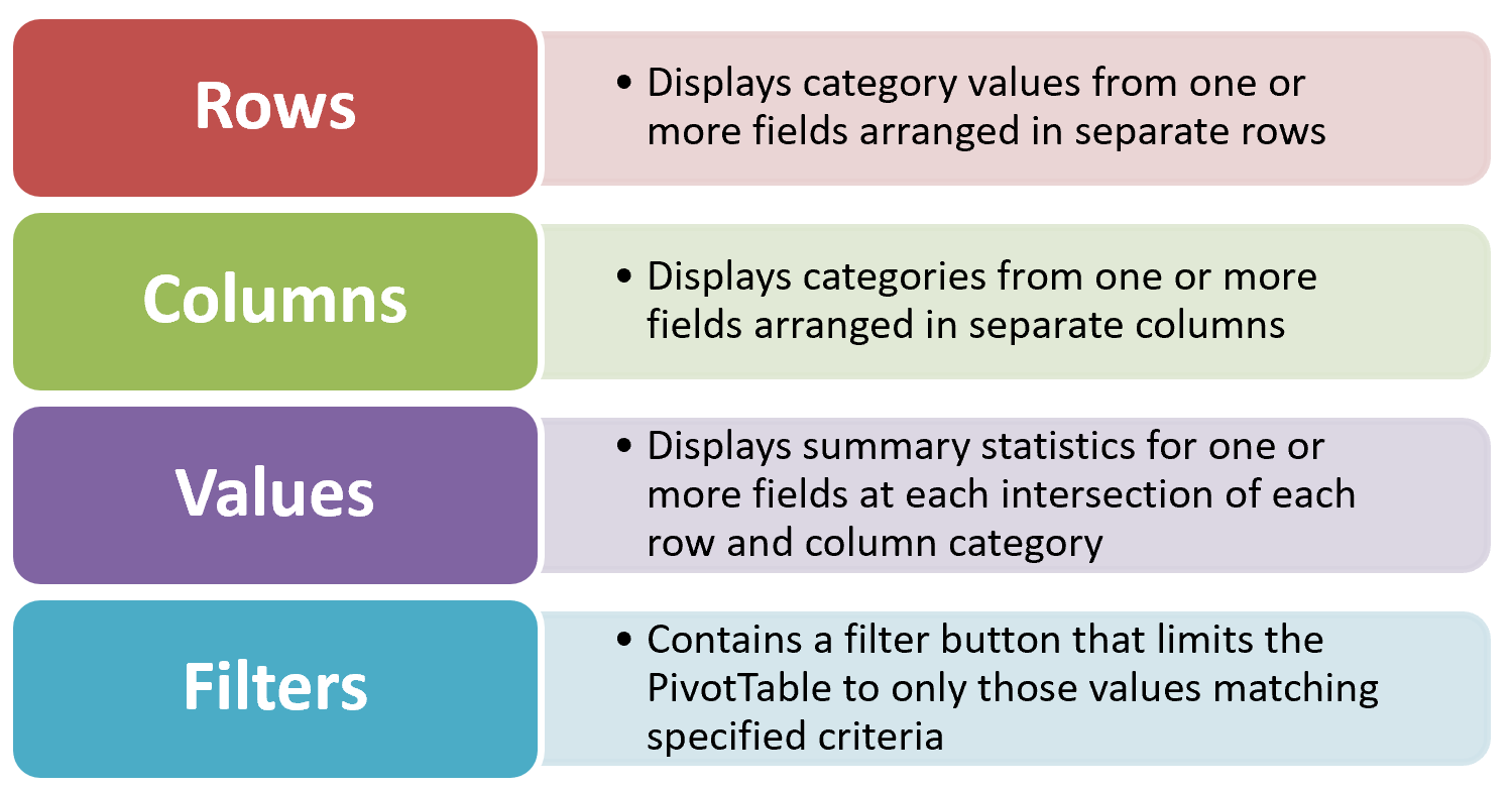
When you pull table data into a PivotTable there are four main area fields: Rows, Columns, Values, and Filters. The Rows and Columns fields can interchange quickly to summarize the data in different ways or to run new reports based on the question or criteria being asked. The Value field is data from the table that can be calculated, or that contain values that the PivotTable will summarize. The Values field has multiple settings to choose how you want to calculate the data; SUM, COUNT, AVERAGE, MIN, MAX, and can even show the displayed values as a percentage of the total, column total, grand total, and so on. Lastly, is the Filters area, which restricts the PivotTable to only show the values matching specified criteria.

Four Primary PivotTable Areas:

Figure 5.49 Four Primary PivotTable Areas

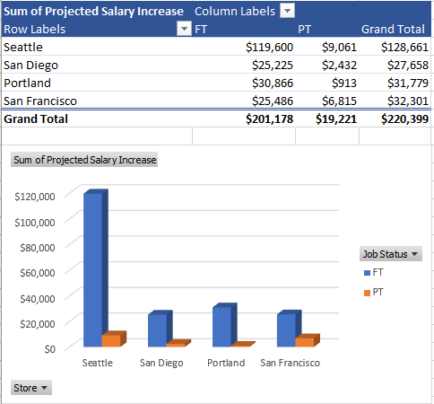
In our situation, shown below, we will create a PivotTable to summarize employee data to show Projected Salary Increases, for both Part-Time (PT) and Full -Time (FT) employees for all store locations.

Figure 5.50 Parts Of A PivotTable

Follow the below steps to explore and build a PivotTable report.

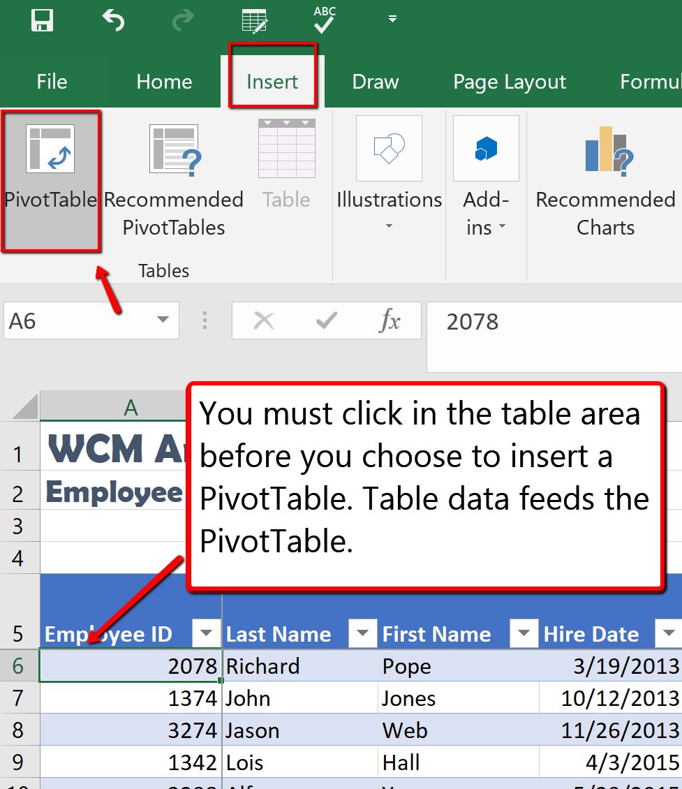
1. Click the EmployeeData sheet. Click anywhere in the table area.
2. From the Insert tab, choose PivotTable.

Figure 5.51 Insert PivotTable

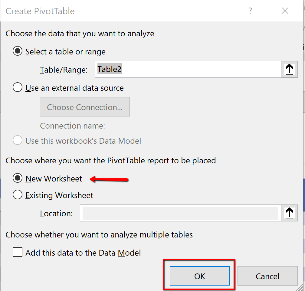
3. From the Create PivotTable dialogue box, make sure the PivotTable report will be placed in a New Worksheet, and click OK.

Figure 5.52 Create PivotTable Dialogue Box

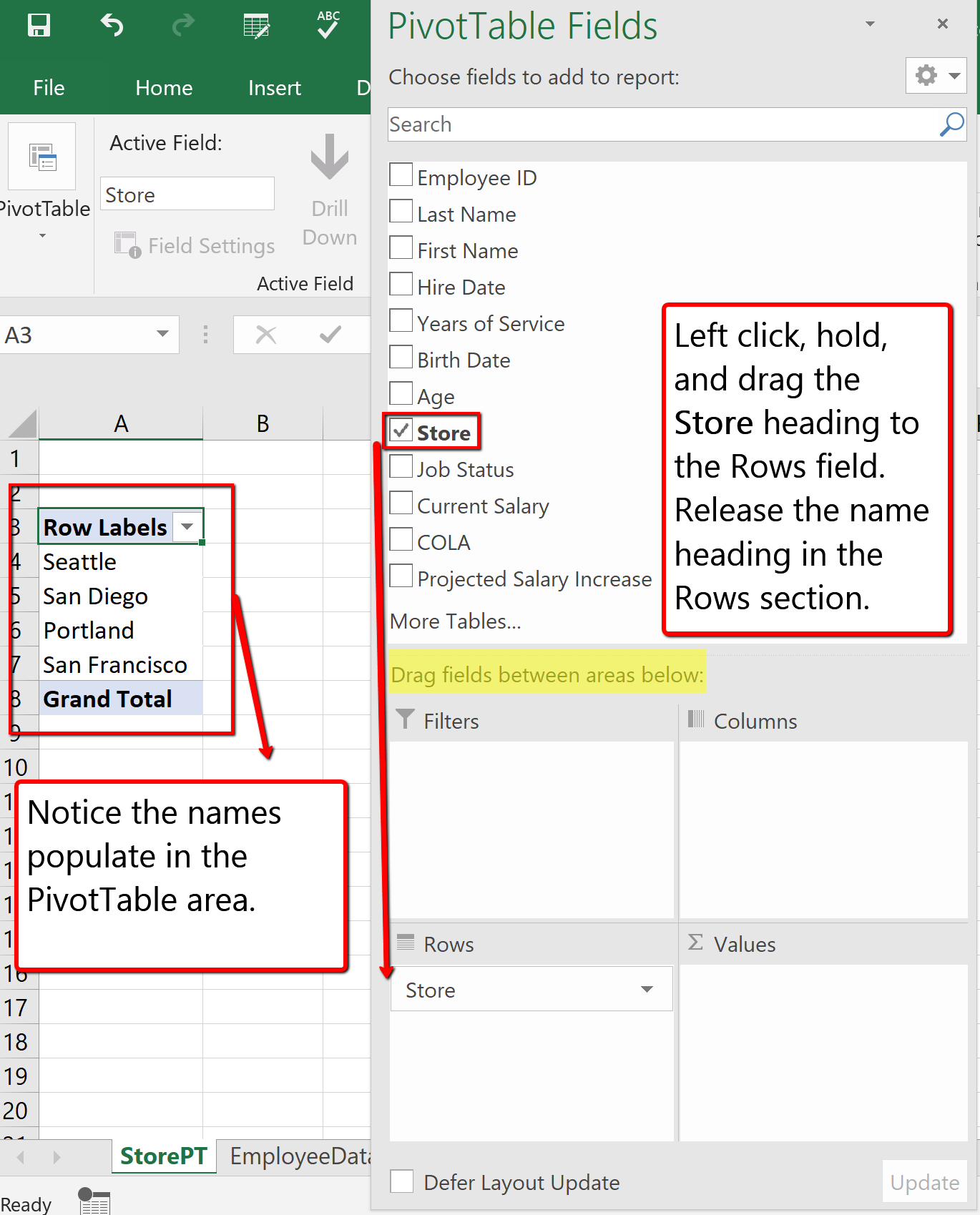
4. Notice a new sheet (Sheet1) is inserted, at the bottom of the workbook, that contains the PivotTable1 area and fields dialogue box. Rename the default name (Sheet 1) to StorePT.

Figure 5.53 PivotTable Window

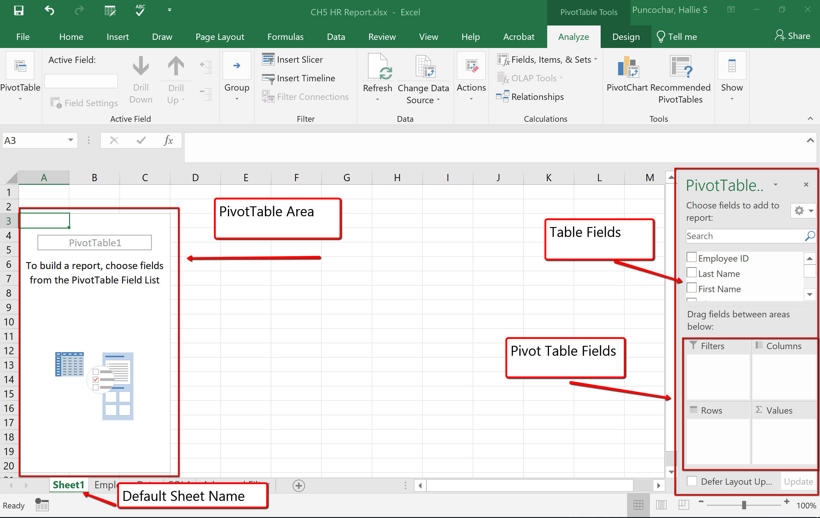
5. From the PivotTable pane, drag and drop the Store heading to the Rows section of PivotTable field area.

Figure 5.54 PivotTable Row Selection

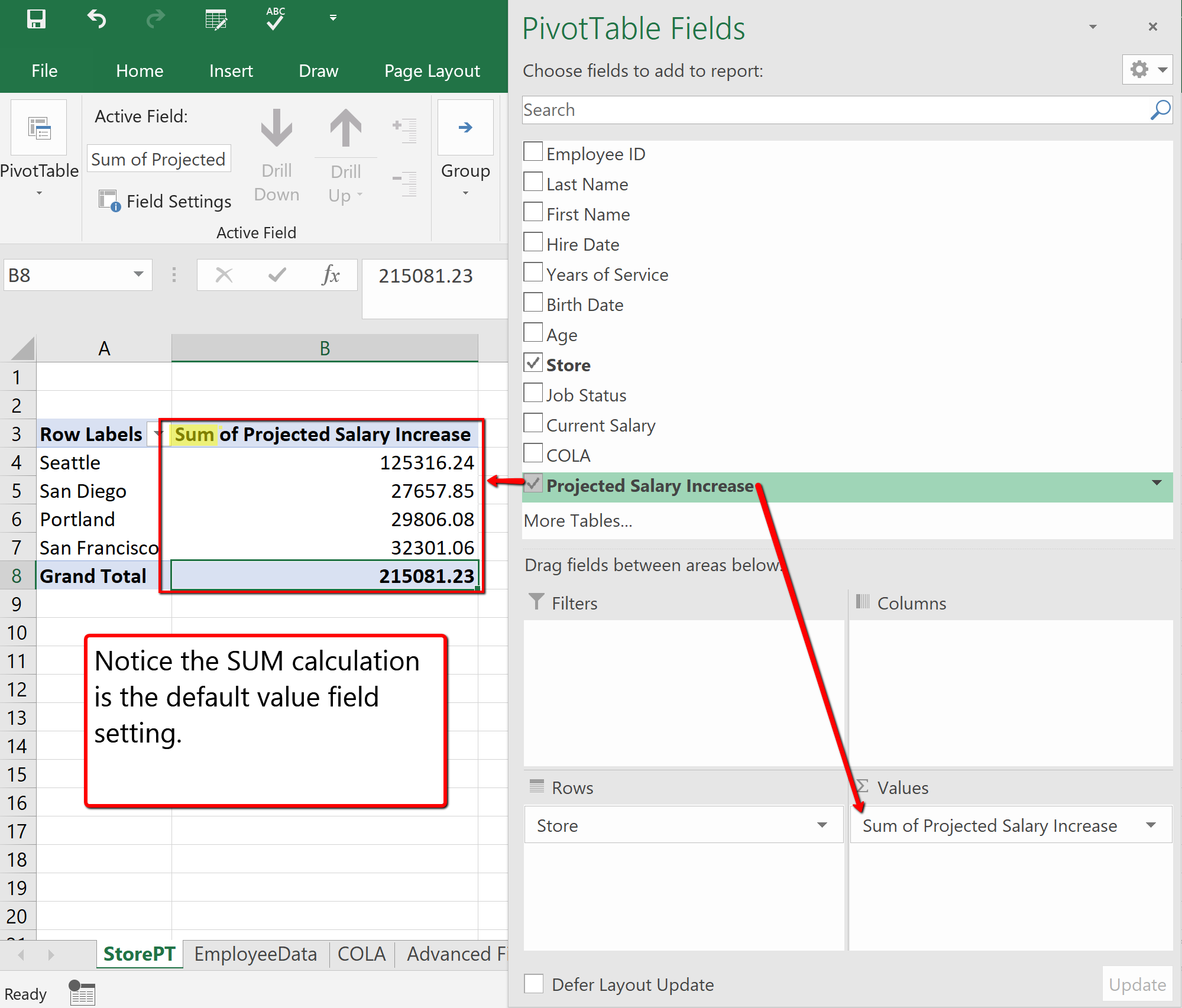
6. From the PivotTable fields list drag and drop the Projected Salary Increase heading to the Values section.

Figure 5.55 PivotTable Value Selection

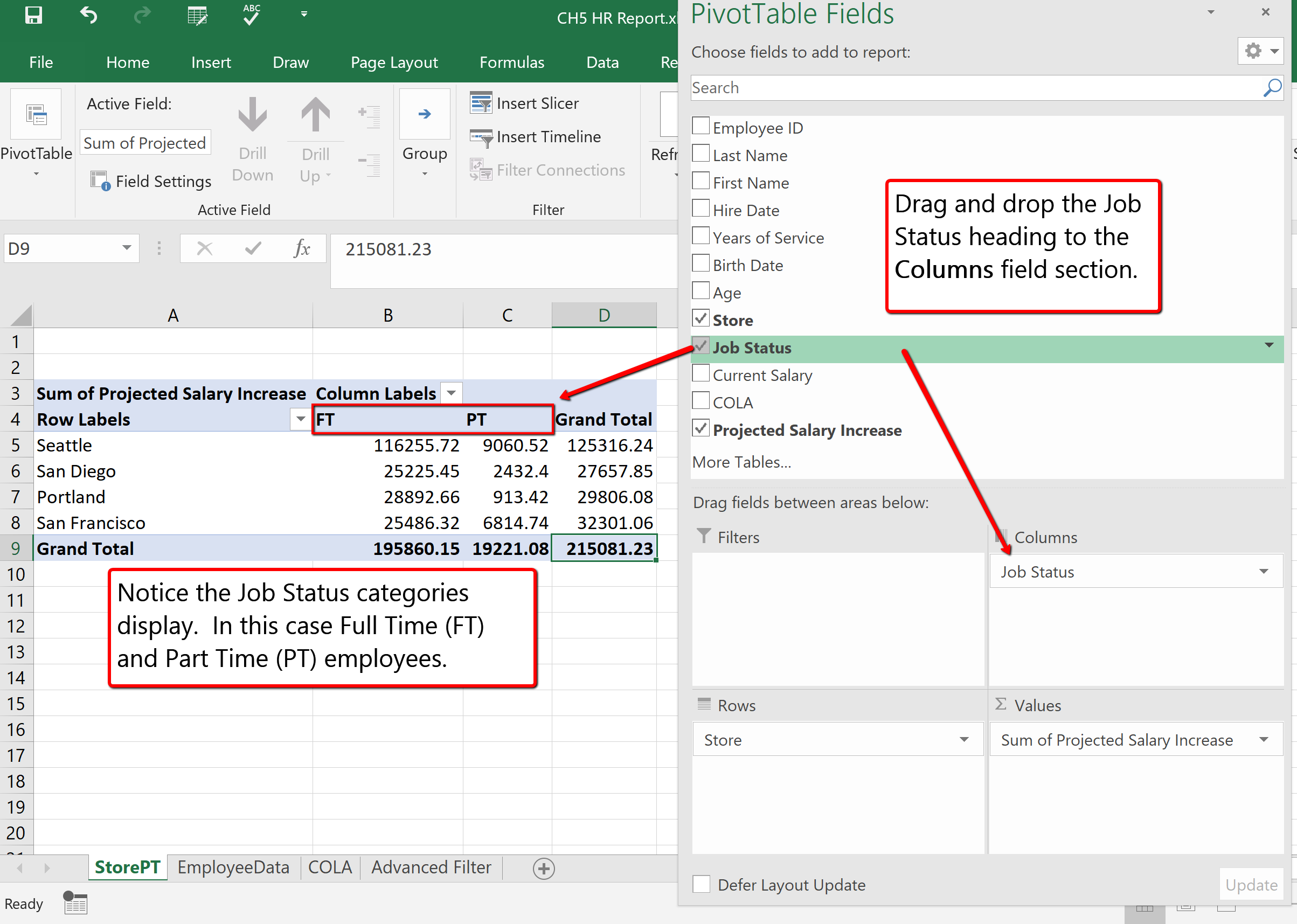
7. Drag and Drop the Job Status heading to the Columns field section. Notice the Job Status categories display. In this case, displaying Full-Time (FT) and Part-Time (PT) employees.

Figure 5.56 PivotTable Columns Selection

FORMATTING PIVOT TABLES

After creating a PivotTable and adding the fields that you want to analyze, you may want to enhance the report to include slicers, or graphs and or format the data to make it easier to read and scan for details. When clicked in the PivotTable area you will see a contextual tab appear on the ribbon, containing PivotTable Tools and two specific tabs; Analyze and Design. Mac Users: there is not a “PivotTable Tools” tab but you will see two tabs named: PivotTable Analyze and Design. They are only visible when you have clicked inside the PivotTable area.

The Analyze tab contains tools specifically for examining data, for example, the ability to insert Slicers, or PivotCharts. The Design tab contains tools that specifically tie to how the table and data visibly display. For example, when you have a lot of data in your PivotTable, it may help to show banded rows or columns for easy scanning or to highlight important data to make it stand out.

Follow the below steps to add format the PivotTable, and add a PivotChart.

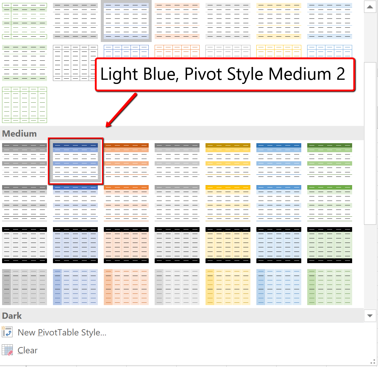
1. Click in the PivotTable. From the PivotTable Tools choose the Design tab.
2. In the PivotTable Styles gallery select the Light Blue, Pivot Style Medium Style 2 format.

Figure 5.57 Light_Blue Medium Style Pivot 2

3. To format the PivotTable numbers, select B5: D9. Click the Home tab. Apply the Currency number format and decrease the decimal place to zero decimals.

(The alternative method to number formatting in a PivotTable is to expand the menu on value field; Sum of Projected Salary Increase. Click the Value Field Settings. Choose Number Format and apply the desired number format option. Mac Users should click the small circle with an “i” next to “Sum Projected Salary Increase” in the Values section then click the Number button to change the Number Format. )

NOW LET’S CREATE A PIVOTCHART!

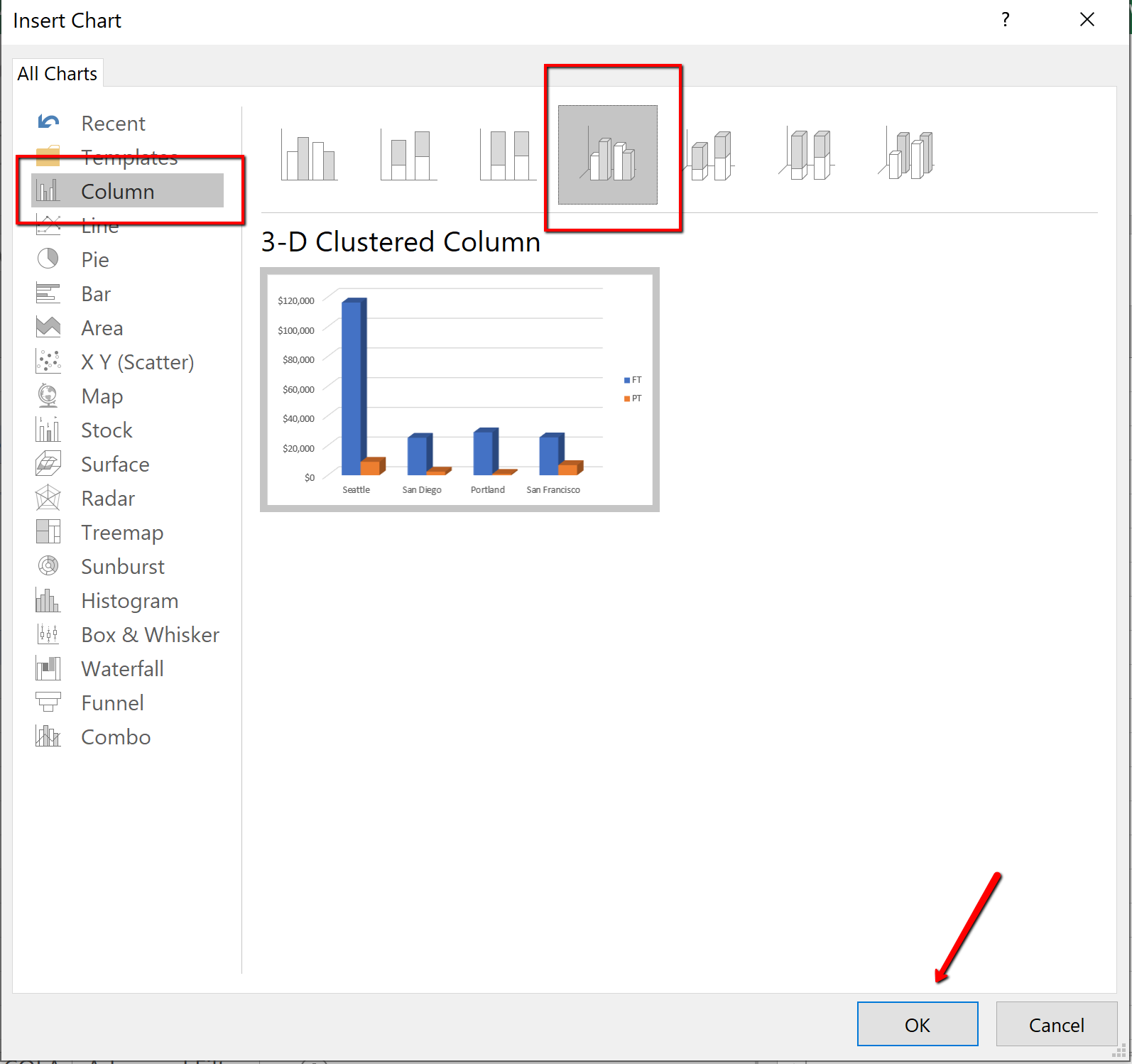
4. Click in the PivotTable. Click the Analyze tab. Choose the PivotChart button on the Ribbon.
5. From the listed chart types, choose Column. And select the 3D Clustered Column option. Click OK.

Mac Users: Only a basic, 2D column chart is available when clicking the Pivot Chart button. In order to select a different chart type, such as the 3D clustered column option, you must do the following:

• • • Click on the 2D chart that was just inserted
    • Click the Design tab on the Ribbon
    • Click the Change Chart Type button
    • Select the 3D Clustered Column option

Figure 5.58 3D Clustered_Column Chart

6. Move the PivotChart under the PivotTable area. Resize accordingly. Save your work.

Note the formatting changes in the new chart below. The “Job Status” and “Store” buttons are column and row “filters” for the Pivot Chart.

Mac Users: Excel for Mac does not insert these formatting changes within a Pivot Chart. You can add a chart title by clicking the “Add Chart Element” button from the Design tab. It is not possible to add the “chart filter” buttons as shown in Figure 5.59. The filters on the pivot table can be used to also filter the columns and rows in the Pivot Chart.

Figure 5.59 PivotTable Solution

SUBTOTALS

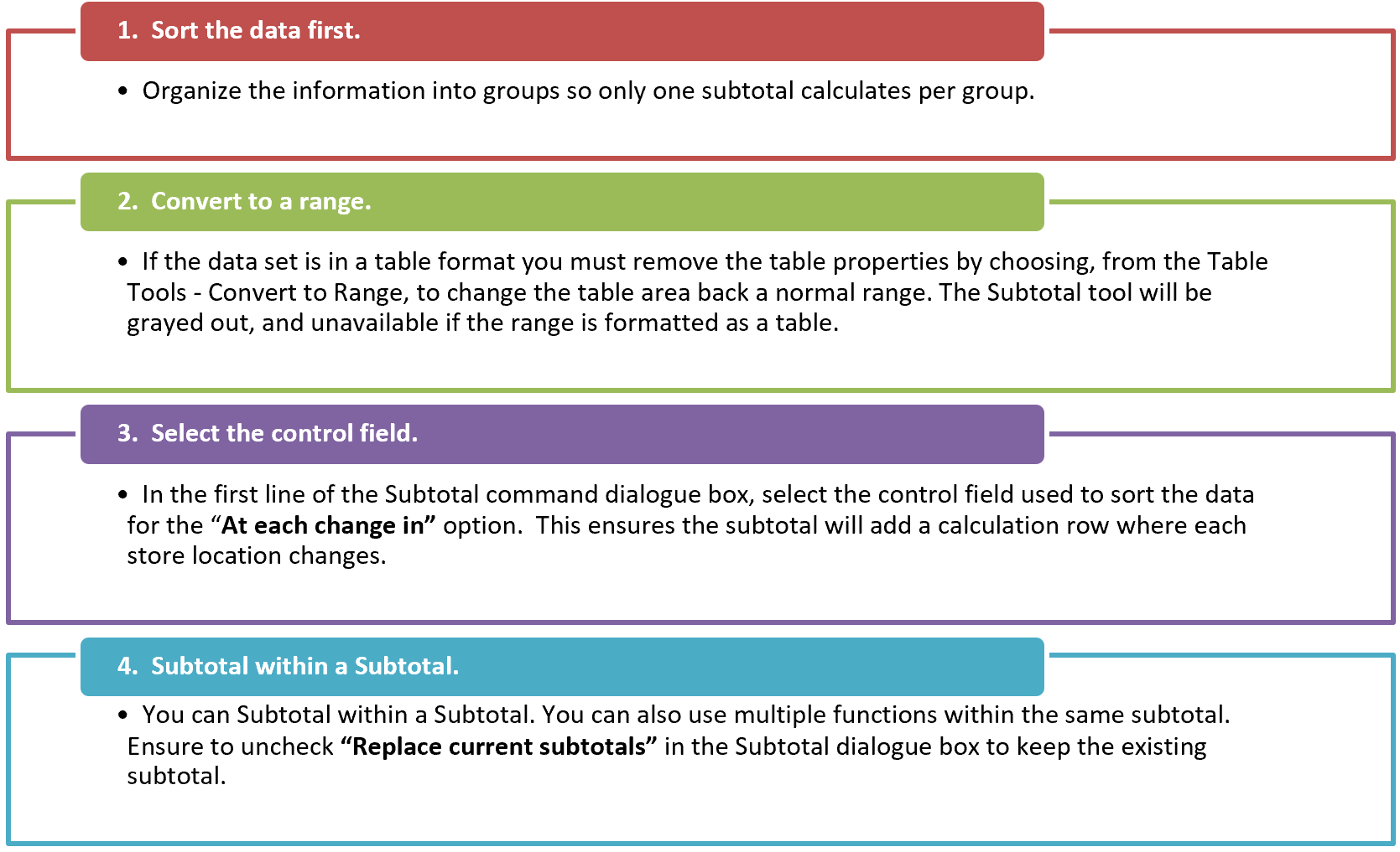
Another way to summarize data is by using subtotals. Analyzing a large data range usually includes making calculations on the data. You can summarize the data by applying summary functions such as COUNT, SUM, and AVERAGE to the entire organized range of information. Subtotals, in general, are summary functions applied to parts of an organized data range.

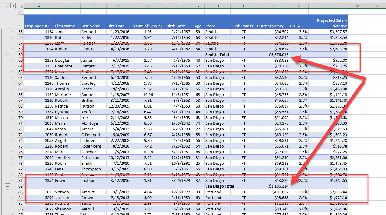
For example, you can SUM Current Salaries for employees from each Store location. To subtotal the information the data must first be sorted by the Store field. For subtotals, the field that you sort is referred to as the control field. For example, if you choose the Store location as your control field, all of the Seattle, San Diego, Portland, and San Francisco entries will be grouped together within the data range. The SUM function then can be applied to SUM the Current Salary fields for each Store location. Excel calculates and displays the subtotal each time the Store location changes.

A new row containing a subtotal of that particular location will be inserted, and wherever the field changes a value will display; a subtotal group of records. Excel updates the subtotal automatically when the control field is changed. In theory, when subtotaling, you are adding a calculation row to the set of data. Adding rows that total information in the middle of a table would compromise the integrity of data in the table. The table tools would look at the total as a record, not a calculation. Therefore the Subtotal feature cannot be used in tabling, and can only be applied to a normal range of data. You must convert all tables to a range prior to subtotaling.

Multiple functions can be applied within the same Subtotal. For example, we will explore how you can SUM Current Salary’s and also provide the AVERAGE Current Salary for each Store location within the same Subtotal. Note Subtotal data can also be filtered.

The best practice when subtotaling is to follow four rules:

Figure 5.60 Subtotal Rules

Follow the below steps to Subtotal the Employee Data and provide a total Current Salary per Store.

1. Select the Employee Data sheet. If necessary clear any filters applied to the data by clicking the Data tab and choosing the Clear filter option.
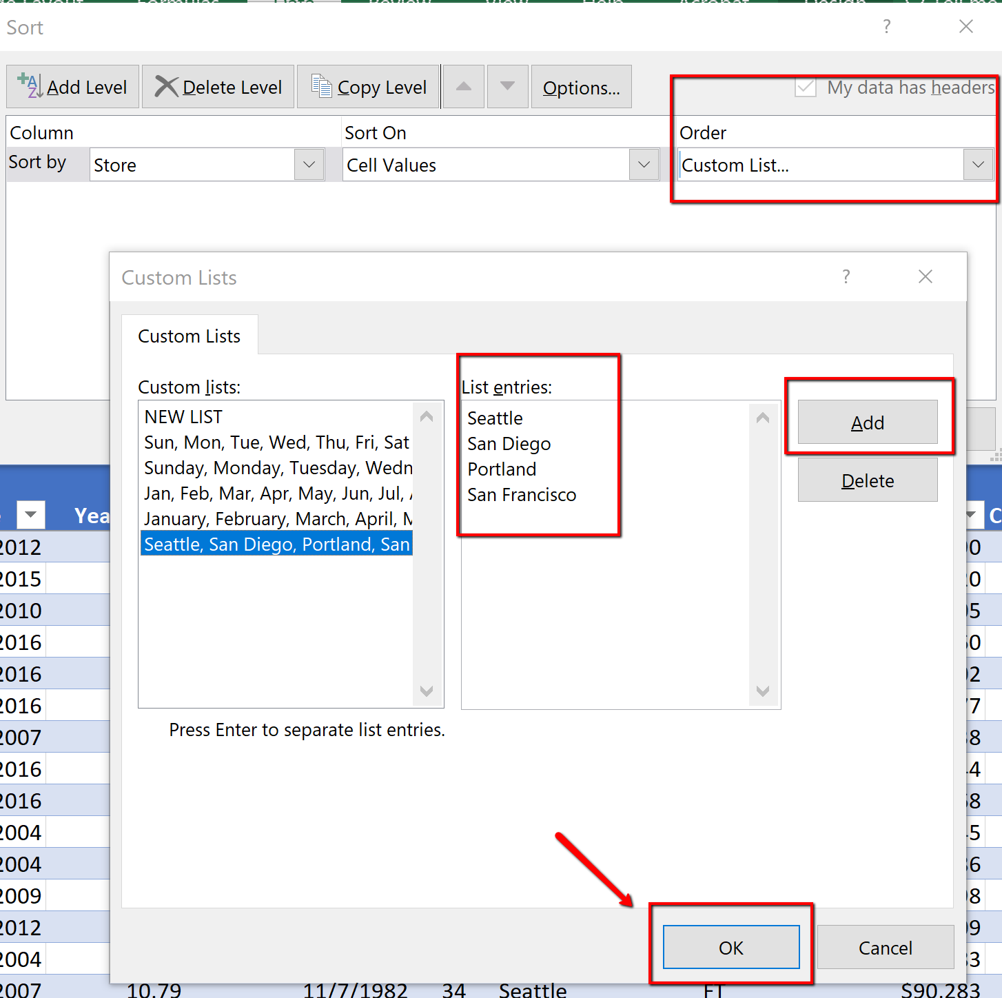
2. From the Data tab, choose Sort button. Sort the Store Location, using the preferred Custom List order of Seattle, San Diego, Portland, and San Francisco. If the list we set up previously is not available type the entries in the List entries area. Choose Add, and then OK.

Figure 5.61 Custom Sort, Custom List Dialogue Box.

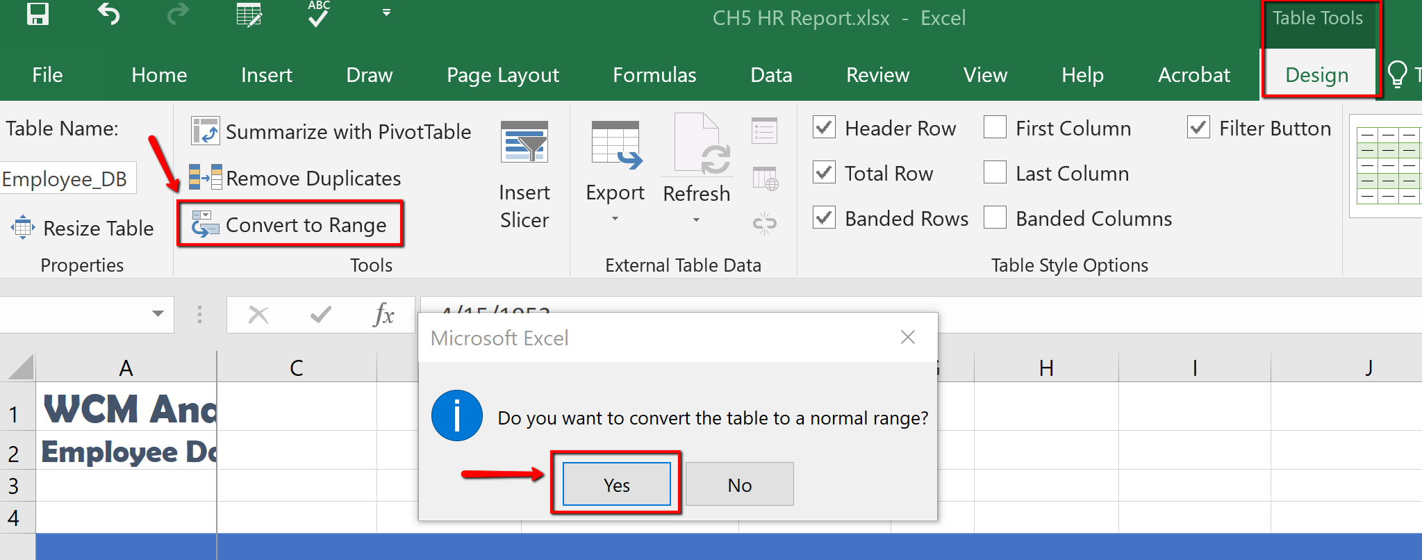
3. Choose the Table Tools Design tab. Mac Users: just click the “Table” tab.

     Select “Convert to Range.” Excel will display a message asking if you really want to convert the table back to a normal range. Choose Yes.

Figure 5.62 Convert To A Range

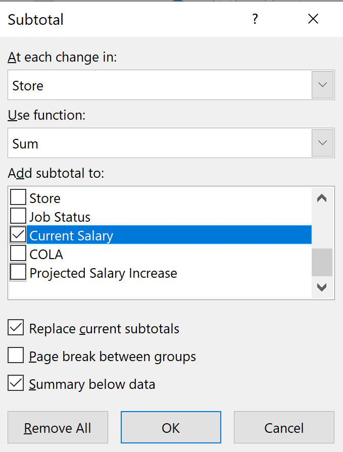
4. Click the Data tab, in the Outline group find and select the Subtotal Command. (Notice the heading row no longer has filters buttons. The data looks like a table but is not a table. The table tools are not active, and the information is a normal range.)
5. In the Subtotal dialogue box, choose the Store field in the “At each change in.” For the “Use Function,” choose Sum, and only check Current Salary. Click OK.

Figure 5.64 Subtotal Dialogue Box

6.  Notice the Current Salary column is totaled, per location. Save your work.

Figure 5.65 Subtotal Solution

SUBTOTAL OUTLINE VIEW

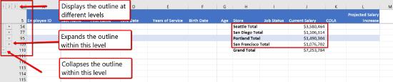
The Outline views, located on the left side panel, show summary statistics. The Outline tool, with levels, allows you to control the expanse of detail displayed in the worksheet. The EmployeeData worksheet has three levels in the outline of its data range:

• Level 1, displays only the grand totals.
• Level 2, displays the total spent at each Store.
• Level 3, displays the total Salary.

Figure 5.66 above shows the Level 3 Outline, all the employee detail per store location. Clicking the outline buttons located to the left of the row numbers lets you choose how much detail you want to see in the worksheet. (Note that the three level numbers are at the top left side of the worksheet, just below the Name box.)

You will use the outline buttons to expand and collapse different sections of the data range.

1. Click level 1. Notice it displays the Grand Total.
2. Click level 2. Notice the totals for all store locations are displayed.

Figure 5.66 Subtotal Outline Level 2

ADDING A SUBTOTAL WITHIN A SUBTOTAL

As mentioned at the beginning of the section, you can use multiple functions within the same subtotal. We will now explore how you can SUM Current Salary’s and also provide the Average Current Salary for each Store location within the same Subtotal.

1. Click within the Subtotal data, go to the Outline, click Level 3, to display all the subtotal data.
2. From the Data tab, and click Subtotal.
3. In the Subtotal dialogue box, select the Store field for the “At each change in:” option.
4. In the “Use function:” section select to display the Average.
5. Only check the Current Salary field in the “Add subtotal to section:”. (Note Excel will default check something in this area. Uncheck any other fields.)
6. Uncheck “Replace current subtotals”; we do not want to replace the current subtotal summing the Current Salary.
7. Click OK

Figure 5.67 Subtotal Within A Subtotal

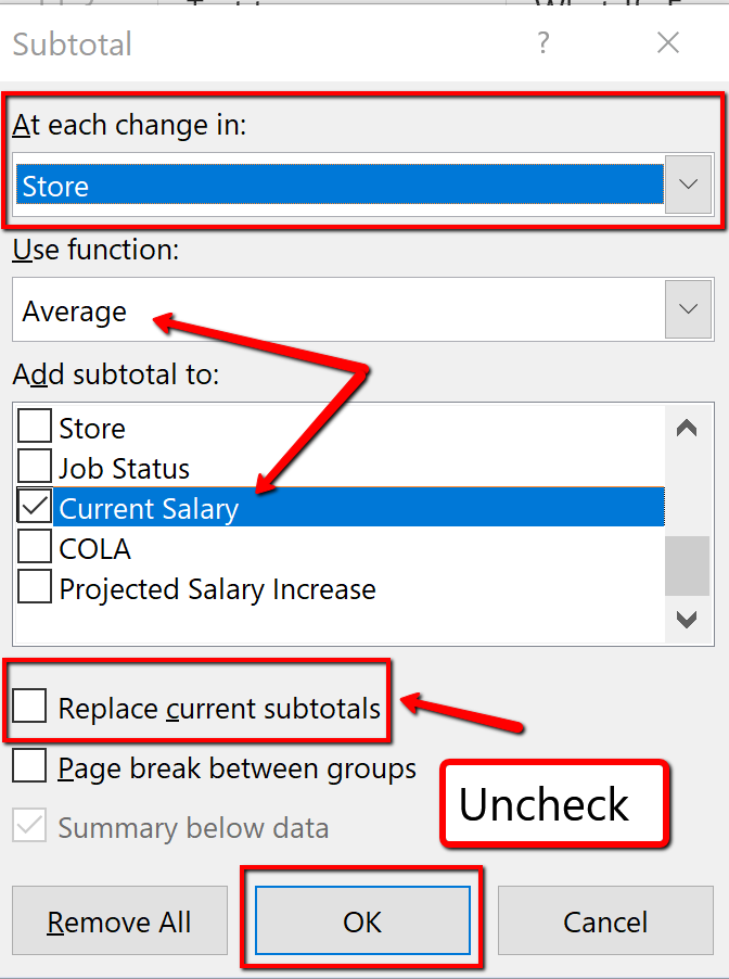
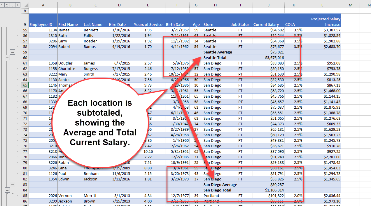
8. Notice each location is now subtotaled showing the Average and Total Current Salary. Excel has also added 4th level to the Outline, accounting for the Averages. Save your work.

Figure 5.68 Solution, Subtotal Within A SubtotalKey Takeaways

Key Takeaways

• A table is made up of a data set that is organized into columns and rows representing fields and records, such as employee information.
• You can create a table by clicking formatting the data set as a table, or using the Insert Table feature.
• Excel offers pre-built table styles, and options to choose from to format a table.
• You can add records (rows) and our fields (columns) to a table. You can then sort to reorganize your data.
• Freezing heading keeps your column headings displayed while you scroll through your table data.
• You can use the filter arrows in the table headings to sort by a single column. When sorting by more than one field, use the Custom Sort option.
• Custom List Sorts can be used when a field needs to be sorted in a special way.
• A slicer is a visual filter button (object) used to filter data in an Excel table. Each unique value in the field is a button.
• A PivotTable is an interactive table that summarizes data from a data source such as a data range or an Excel table.
• The Subtotal tool includes summary statistics for each group of records. Excel organizes subtotals using an outline that can be expanded or contracted to view or hide details about the data.

“5.2 Intermediate Table Skills” by Hallie Puncochar, Portland Community College is licensed under CC BY 4.0