15.5: Styles Group

Last updated
Save as PDF

Page ID: 13680

\( \newcommand{\vecs}[1]{\overset { \scriptstyle \rightharpoonup} {\mathbf{#1}} } \) \( \newcommand{\vecd}[1]{\overset{-\!-\!\rightharpoonup}{\vphantom{a}\smash {#1}}} \)\(\newcommand{\id}{\mathrm{id}}\) \( \newcommand{\Span}{\mathrm{span}}\) \( \newcommand{\kernel}{\mathrm{null}\,}\) \( \newcommand{\range}{\mathrm{range}\,}\) \( \newcommand{\RealPart}{\mathrm{Re}}\) \( \newcommand{\ImaginaryPart}{\mathrm{Im}}\) \( \newcommand{\Argument}{\mathrm{Arg}}\) \( \newcommand{\norm}[1]{\| #1 \|}\) \( \newcommand{\inner}[2]{\langle #1, #2 \rangle}\) \( \newcommand{\Span}{\mathrm{span}}\) \(\newcommand{\id}{\mathrm{id}}\) \( \newcommand{\Span}{\mathrm{span}}\) \( \newcommand{\kernel}{\mathrm{null}\,}\) \( \newcommand{\range}{\mathrm{range}\,}\) \( \newcommand{\RealPart}{\mathrm{Re}}\) \( \newcommand{\ImaginaryPart}{\mathrm{Im}}\) \( \newcommand{\Argument}{\mathrm{Arg}}\) \( \newcommand{\norm}[1]{\| #1 \|}\) \( \newcommand{\inner}[2]{\langle #1, #2 \rangle}\) \( \newcommand{\Span}{\mathrm{span}}\)\(\newcommand{\AA}{\unicode[.8,0]{x212B}}\)

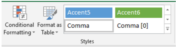
The Styles Group allows the user to use some predetermined styles consisting of fonts and colors to determine the appearance of the cell. Conditional Formatting allows the user to program Excel to change the color of selected cells based upon the conditions in a cell. Selecting Conditional Formatting will launch a drop-down menu allowing the user to customize the specific conditional formatting.

Conditional Formatting

When preparing a large financial report, and excel user may want to make specific cell ranges more recognizable to focus the attention of their audience; perhaps they would like to highlight specific areas indicating profits visually and also showcase areas of financial losses another. The user can use Conditional Formatting to have Excel automatically label or create graphics for cells based upon properties they specify.

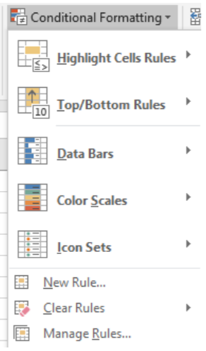
Selecting Highlight Cell Rules will apply the specific cell shading to selected cells with values either greater than, less than, between, equal to, the text contains, or a specific date, or duplicate values. Once the specific measure is selected, a new dialog box will launch allowing the user to input their specific value and the cell shading color that would be associated with it.

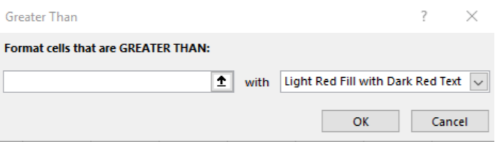
Highlight Cell Rules: Typically, an Excel user would utilize Highlight Cell Rules to program Excel to display certain cells to stand out to the user. For example, a CFO may use conditional formatting to program cells with negative balances to be colored red to stand out to their boss.

Top/Bottom Rules: These selection options allow the user to highlight the Top 10 items in a list, the Top 10%, Bottom 10 items, Bottom 10%, Above Average, and Below Average. In addition, any custom rules can be created as well.

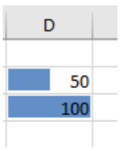
Data Bars: Once the user has set rules for Conditional Formatting, Excel allows for multiple ways to display the data. Using the Data Bars feature of Conditional Formatting, users can create a fill a cell with a chosen color that fills relative to the data in the cell. For example, for the purposes of simplicity, a user could have two data points in two different cells, 50 and 100. Using the Conditional Formatting with Data Bars, the user can create a visual that compares the two data points in the cells visually. The number “50” makes the cell appear half-filled, while “100” fills the entire cell. Colors can be changed.

The user can always program the data bars to calculate differently by selecting the last option in the drop-down menu, More Rules.

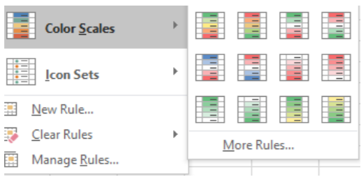
Color Scales: In addition to Data Bars, the user can determine multiple color gradients to appear in cells based upon the Conditional Formatting rules. The cell can be shaded completely, or outlined depending on the user’s preferences. Like Data Bars, the user can always provide more detail as to what data is displayed in the Color Scales by selecting “More Rules”. Below the gradient options.

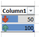
Icon Sets: In addition to colors, Excel users can display specific images or symbols in cells based upon their parameters and the data in the cell. There are a variety of arrows and shapes that can be associated with cells.

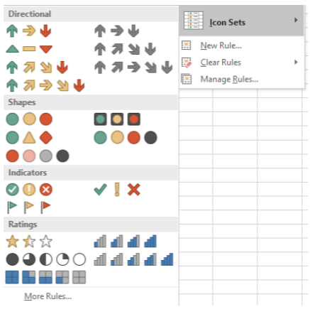
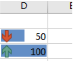
Using the previous example of placing “50” in one cell and “100” in the one below it, using Icon Sets, the user can place pictures (such as arrows) in the cells to indicate their value with or without the shading properties from the data bars. In addition to the multiple graphic options, users can create custom rules by selecting the “More Rules” field in the Icon sets drop-down menus to determine how each cell appears. Depending on the rules established, the arrows, shapes, indicators or ratings will change.

Format as Table

While Excel is organized to present information in a grid-like table, the cells can be more precisely configured to be organized into a separate table format. To set up a table, select the cells that will compose the table and click the “Format as Table” icon in the styles group. A dropdown arrow will launch a variety of table shading styles to select in terms of color and gradient (Light, Medium, and Dark). Formatting the table will allow for each row to be shaded in alternating colors to best differentiate the rows, and a header row will be placed at the top of the table. The header row allows the user to label the data in each column and also perform a variety of data sorting activities.

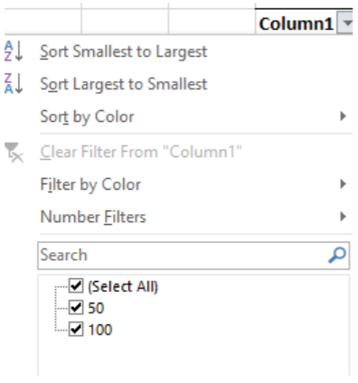
By clicking on the downward arrow on the right of the header row cell, a dropdown box will launch a variety of data manipulation options. Users can sort the data in that row from smallest to largest, largest to smallest, sort by color (if using conditional formatting), filter by color, and create filters for numbers in a cell. Filters only display text that the user specifies. For example, in a table with multiple numbers ranging from 1 to 10, filtering numbers “1” and “3” will only display those numbers in the table. The rest of the numbers will disappear until the user removes the filter, which is also located in the drop-down menu. In addition, the user can select the specific numbers to filter.

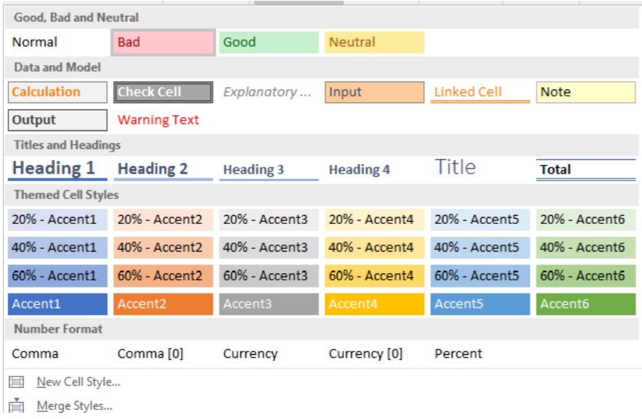
Cell Styles

The last option in the Styles Group is the Cell Styles icon. . Like Microsoft Word, Excel provides a number of preset styles with different colors and fonts. Instead of styles relating to paragraphs or sentences, they relate to individual cells instead. Selecting Cell Styles will load a dropdown menu that provides a variety of cell shading options, different font and heading styles, and style themes in addition to number formats. Using styles allows the user to create standard cell properties across their document by using the same cell styles.