1.2.2.13: Speed of Processing

Speed of processing

How does one measure the speed of, say a Porsche 911? One could measure the time that it takes to drive a given distance e.g. the 900 km from Cape Town to Bloemfontein takes 4’/2 hours (ignoring speed limits and traffic jams). Alternatively, one can indicate how far it can be driven in one standard time unit e.g. the car moves at a cruising speed of 200 km/hour.

In the same way, one can measure the speed of the CPU by checking the time it takes to process one single instruction. As indicated above, the typical CPU is very fast and an instruction can be done in about two billionths of a second. To deal with these small fractions of time, scientists have devised smaller units: a millisecond (a thousandth of a second), a microsecond (a millionth), a nanosecond (a billionth) and a picosecond (a trillionth).

However, instead of indicating the time it takes to execute a single instruction, the processing speed is usually indicated by how many instructions (or computations) a CPU can execute in a second. This is exactly the inverse of the previous measure; e.g. if the average instruction takes two billionths of a second (2 nanoseconds) then the CPU can execute 500 million instructions per second (or one divided by 2 billionths). The CPU is then said to operate at 500 MIPS or 500 million of instructions per second. In the world of personal computers, one commonly refers to the rate at which the CPU can process the simplest instruction (i.e. the clock rate). The CPU is then rated at 500 MHz (megahertz) where mega indicates million and Hertz means “times or cycles per second”. For powerful computers, such as workstations, mainframes and supercomputers, a more complex instruction is used as the basis for speed measurements, namely the so-called floating-point operation. Their speed is therefore measured in megaflops (million of floating-point operations per second) or, in the case of very fast computers, teraflops (billions of flops).

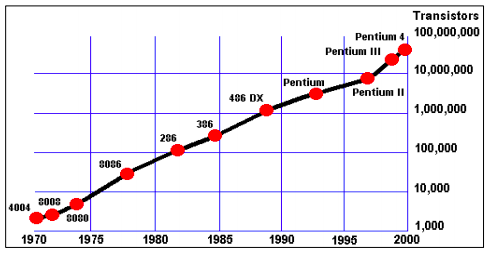
In practice, the speed of a processor is dictated by four different elements: the “clock speed”, which indicates how many simple instructions can be executed per second; the word length, which is the number of bits that can be processed by the CPU at any one time (64 for a Pentium IV chip); the bus width, which determines the number of bits that can be moved simultaneously in or out of the CPU; and then the physical design of the chip, in terms of the layout of its individual transistors. The latest Pentium processor has a clock speed of about 4 GHz and contains well over 100 million transistors. Compare this with the clock speed of 5 MHz achieved by the 8088 processor with 29 000 transistors!

Moore’s Law (see Figure 2) states that processing power doubles for the same cost approximately every 18 months.

Here's how the various aspects of CPU performance can be understood through agricultural analogies:

 

1. Measuring Speed: The Tractor Analogy

Measuring Speed:

• Porsche 911 Example: Just as you can measure a car's speed by tracking how long it takes to cover a certain distance (e.g., 900 km in 4.5 hours) or by its cruising speed (e.g., 200 km/hour), you can measure a CPU's speed by the time it takes to process a single instruction or by how many instructions it can handle in a second.

Agricultural Analogy:

• Tractor Speed: Imagine you're measuring the speed of a tractor in a field. You could measure how long it takes for the tractor to plow a certain length of a field, or you could measure its operating speed in terms of how many hectares it can plow per hour. Similarly, you can measure a CPU's speed by how many instructions it can process in a given time (like hectares per hour for a tractor) or by the time it takes to execute a single instruction.

 

2. Measuring Units: Efficiency in Farming

Units of Time:

• CPU Time Measurement: For CPUs, measurements are in milliseconds, microseconds, nanoseconds, or even picoseconds. The faster the CPU, the smaller the time unit it operates in.

Agricultural Analogy:

• Harvesting Efficiency: In farming, you might measure how long it takes to harvest a single row of crops or how many rows a harvester can process in a given time. Just as with CPUs, smaller time units (e.g., minutes versus hours) can show greater efficiency. A harvester that can process more rows per hour (smaller time unit) is more efficient, similar to a CPU that operates in nanoseconds being faster than one in microseconds.

 

3. Processing Speed: Output and Capacity

Processing Speed:

• CPU Speed Measurement: CPU speed is often described by how many instructions it can execute per second (e.g., 500 million instructions per second or MIPS) or by the clock rate (e.g., 500 MHz).

Agricultural Analogy:

• Production Capacity: Think of a combine harvester’s capacity to process grain. You can measure its efficiency by how many bushels of grain it can process per hour (akin to instructions per second) or by its operational speed (similar to MHz for a CPU). For example, a combine that processes 500 bushels per hour is analogous to a CPU that performs 500 MIPS.

 

4. Key Performance Factors:

Performance Factors:

• Clock Speed, Word Length, Bus Width: CPU performance is influenced by these factors—clock speed (cycles per second), word length (bits processed at once), and bus width (data moved at once).

Agricultural Analogy:

• Tractor Specifications: Consider a tractor's performance factors:
  • Engine Power (Clock Speed): The engine power determines how fast the tractor can operate, similar to a CPU's clock speed.
  • Width of the Plow (Word Length): A wider plow can cover more ground in one pass, similar to a CPU’s word length which affects how much data can be processed at once.
  • Attachment Size (Bus Width): Larger or more attachments allow the tractor to move more material in a single pass, like the bus width affecting data movement.

 

5. Technological Advancement:

Technological Progress:

• Moore’s Law: Moore’s Law states that processing power doubles approximately every 18 months, reflecting rapid advancements in technology.

Agricultural Analogy:

• Improvements in Machinery: Just as Moore’s Law describes the exponential growth in CPU power, the agricultural industry sees similar advancements with improvements in machinery. For example, the efficiency and capabilities of harvesters, tractors, and irrigation systems have grown rapidly over the years, making farming more productive and efficient.

 

6. Historical Comparison:

Historical Comparison:

• Old vs. New CPUs: Comparing early CPUs (like the 8088) to modern processors (like the latest Pentium), you see significant improvements in speed and complexity.

Agricultural Analogy:

• Old vs. New Machinery: Comparing early farming equipment (such as a basic hand plow) to modern machinery (like advanced combines and tractors), you can see similar leaps in efficiency and capability.

 

In Summary:

Just as measuring the speed and efficiency of agricultural equipment involves tracking how much work it can do in a given time or how quickly it performs tasks, measuring CPU speed involves similar metrics: how many instructions it can process in a second and how quickly it can execute tasks. The evolution of CPUs and agricultural machinery reflects advancements in technology and efficiency, making both sectors more productive and effective over time.

Figure 2. Illustration of Moore’s Law