6.1: Appendix I- Graph theory

Undirected graphs

Graphs are mathematical structures that describe relations between pairs of things. They can be represented by diagrams, where a vertex stands for a thing and an edge for a relation between two things. In the graph of a family tree, for example, the vertices represent the family members and the edges their relationships (Figure 1). Any part of the graph, for example, the nuclear family of father, mother, child and their relations to each other, is a subgraph. Two vertices are adjacent if they are joined by an edge. The two vertices are incident with this edge and the edge is incident with both vertices.

Figure 1. A family tree as a graph

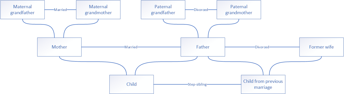
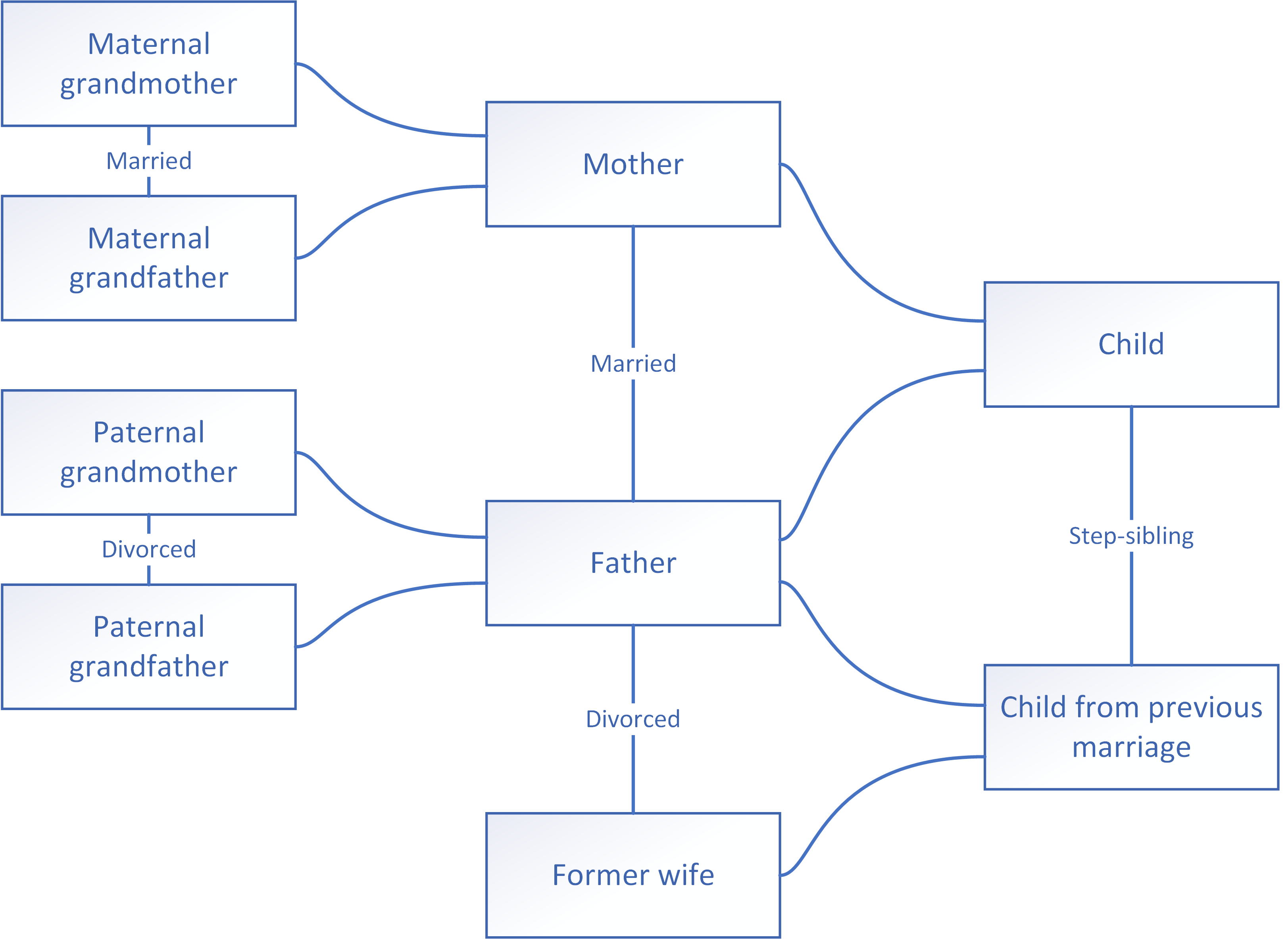
Graph diagrams are dimensionless: the size of a vertex and the length of an edge do not matter either for the vertex and edge or for the whole graph. The size of a graph is measured by the number of edges in it, while the number of vertices is the order of the graph. This means that different arrangements of the vertices and edges in a graph drawing are equally acceptable, so long as they follow a logic that helps legibility (Figure 2). The graphs in Figure 1 and 2 are isomorphic: they have the same vertices and, whenever a pair of vertices in either graph is connected by an edge, the same also holds for the other graph.

The main concern with graph diagrams is that care should be taken that edges do not cross each other in the drawing because this indicates that the graph is planar. Planar graphs have mathematical advantages that relate to the subject of this book (representation of buildings and processes), so you must try and draw your graphs in a way that demonstrates this. Note that a graph may be planar even if you are unable to find an arrangement where no edges intersect. Graph drawing remains a hard task, even with computers. To ensure legibility, do the following in your graphs:

• Arrange the nodes in a logical manner (e.g. in columns, rows or other clusters), without worrying for the size of the drawing or the length of the edges
• Try to have no crossing or overlapping edges, again without worrying about the resulting length or shape of the edges

Figure 2. The same family tree and graph

Properties (including size) can be attached to vertices and edges as labels (textual or visual). The edges of the family tree are labelled with the relationship between the persons represented by the vertices they connect. The default relationship between parent and child is left unlabelled. In general, it is recommended that you use textual labelling rather than visual because it simplifies graph drawing and reading.

Graphs can also be described by adjacency matrices, in which each cell contains the connection between the vertex in the row and the vertex in the column. Table 1 shows if there is a direct connection between the two family members (usually a first-degree relationship). Table 2 shows the relationship as labelled in the graph. Table 2 therefore conveys exactly the same information as the graph drawing, only in a different form.

Table 1. Adjacency matrix of the family tree graph

	Maternal grandmother	Maternal grandfather	Paternal grandmother	Paternal grandfather	Mother	Father	Former wife	Child	Child from previous marriage
Maternal grandmother	×	1	0	0	1	0	0	0	0
Maternal grandfather	1	×	0	0	1	0	0	0	0
Paternal grandmother	0	0	×	1	0	1	0	0	0
Paternal grandfather	0	0	1	×	0	1	0	0	0
Mother	1	1	0	0	×	1	0	1	0
Father	0	0	1	1	1	×	1	1	1
Former wife	0	0	0	0	0	1	×	0	1
Child	0	0	0	0	1	1	0	×	1
Child from previous marriage	0	0	0	0	0	1	1	1	×

Table 2. Adjacency matrix of the family tree graph (labelled)

	Maternal grandmother	Maternal grandfather	Paternal grandmother	Paternal grandfather	Mother	Father	Former wife	Child	Child from previous marriage
Maternal grandmother	×	married	0	0	parent	0	0	0	0
Maternal grandfather	married	×	0	0	parent	0	0	0	0
Paternal grandmother	0	0	×	divorced	0	child	0	0	0
Paternal grandfather	0	0	divorced	×	0	child	0	0	0
Mother	child	child	0	0	×	married	0	parent	0
Father	0	0	child	child	married	×	divorced	parent	parent
Former wife	0	0	0	0	0	divorced	×	0	parent
Child	0	0	0	0	child	child	0	×	step-sibling
Child from previous marriage	0	0	0	0	0	child	child	step-sibling	×

Each vertex in a graph has a degree: the number of edges connected to it. In the family tree example, each grandparent and child vertex has a degree of 3, the mother vertex 4 and the father vertex 6. The former wife, whose parents do not appear in the graph, has a degree of only 2. The degree of a node is a good indication of its importance or complexity. In this case, it is logical that the father node has the highest degree because the family tree focuses on his former and current marital situation. An odd vertex is one with a degree that is an odd number, while the degree of an even vertex is even. A vertex with a degree equal to zero is called isolated, while a vertex with a degree of 1, as the end stations in the metro map from the chapter on symbolic representation (vertices A, H, G and N in Figure 3), is called a leaf.

The degree sequence of a graph is obtained by listing the degrees of vertices in a graph. This is particularly useful for identifying heavily connected subgraphs. In a metro map, for example, it shows not only which vertices are busy interchanges but also their proximity and distribution: which parts of a line present the most opportunities for changing to other lines.

Figure 3. The graph of a metro map

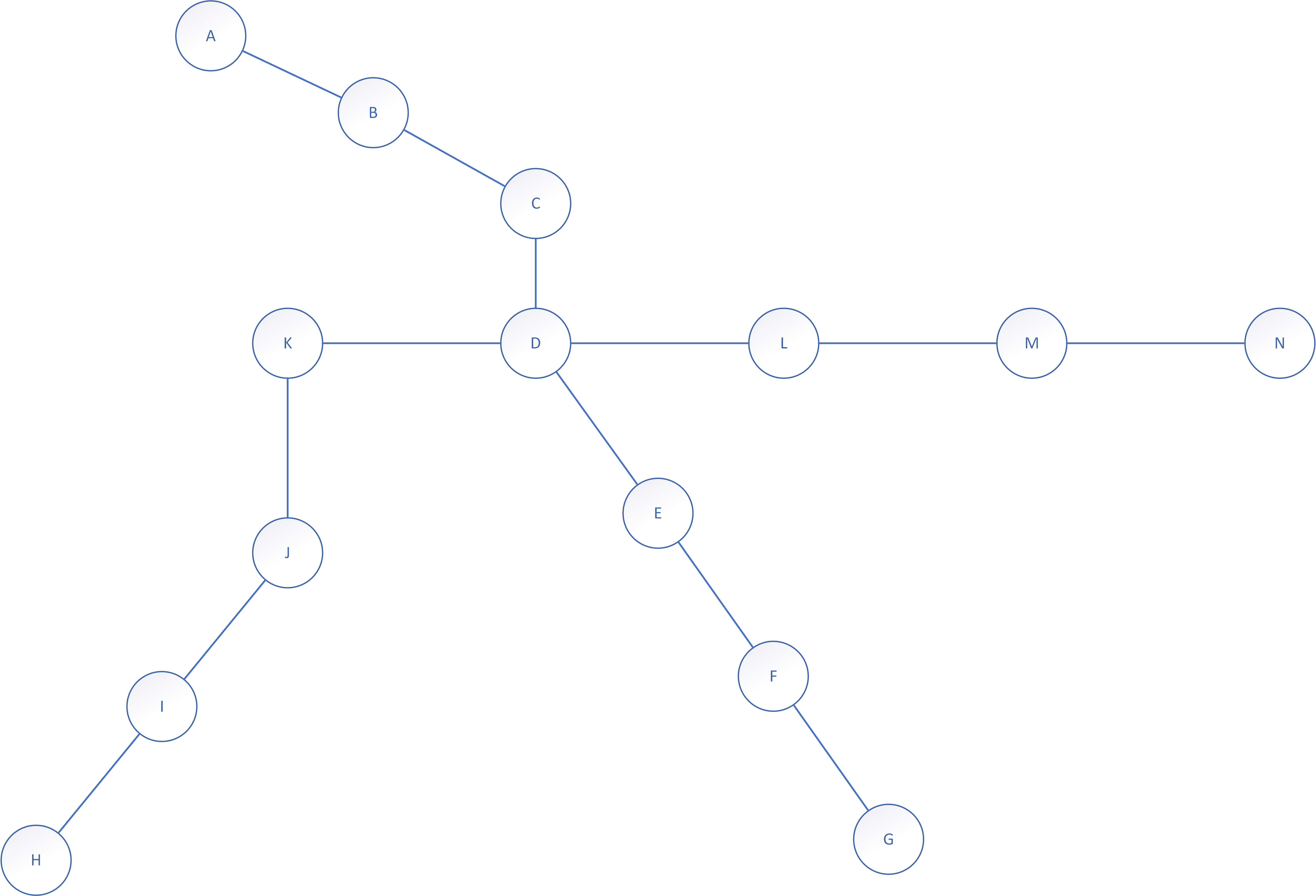
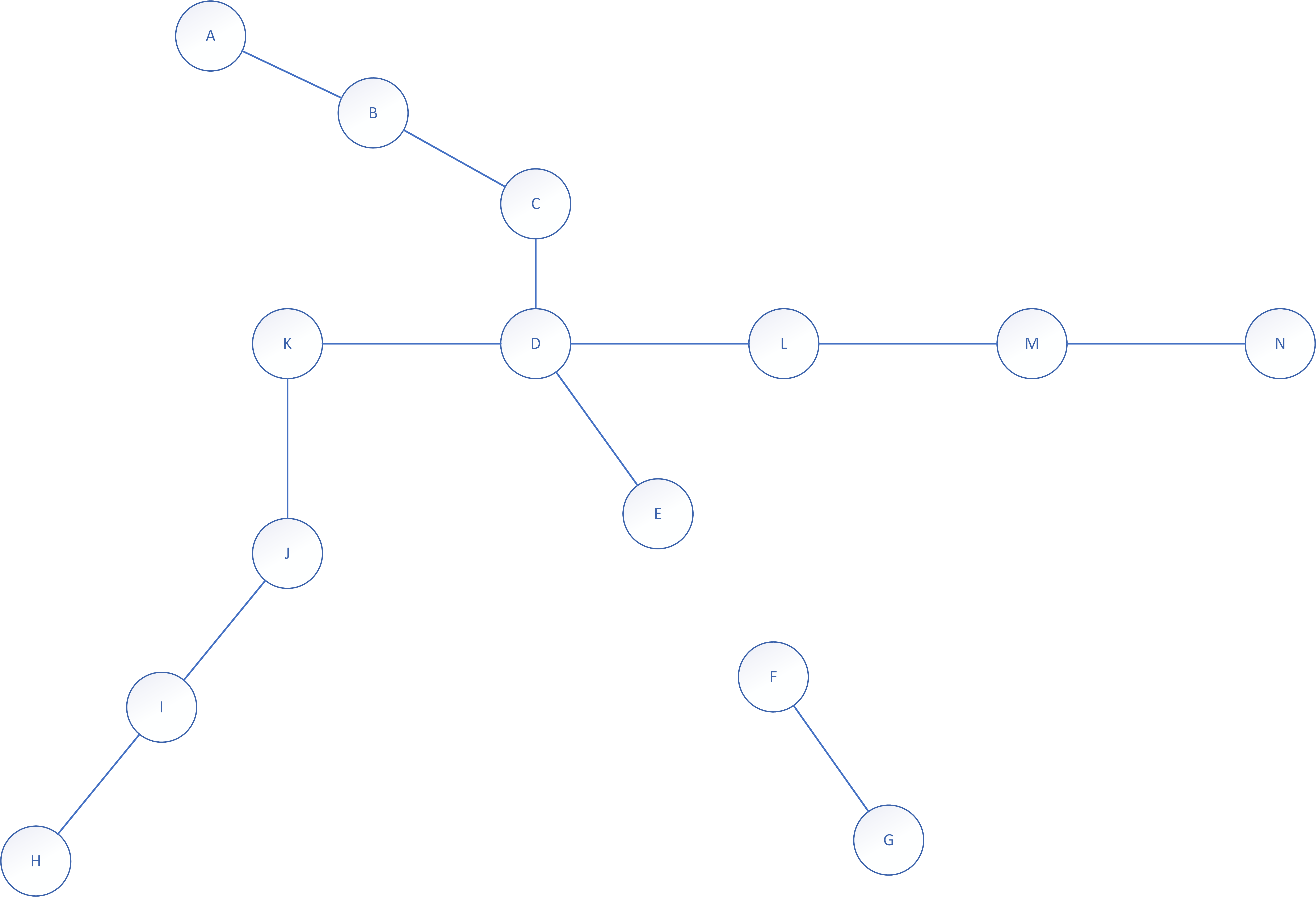
A graph in connected if each of its vertices connects to every other vertex by some sequence of edges and vertices (a walk). The graphs in this book are by definition connected: in a building there is practically always a way to go from one place to another, while processes should be characterized by continuity from beginning to end. In fact, we pay particular attention to interruptions of connectedness, such as bridges and minimal cuts. A bridge is an edge that divides a graph into two separate parts, so its removal renders the graph disconnected. In the family tree, no edge is a bridge. If an edge is removed from it, there are always a connection between two family members it connected. For example, if the two children sever direct communication between them, there is always the possibility to communicate via the father or, more indirectly, through the rest of the family. Such bridgeless graphs hold advantages for communication and continuity: a metro map that is a bridgeless graph means that passengers can reach their destination, even when the connection between two stations is disrupted. In this respect, our metro example is poor: in Figure 3, all edges are bridges. The removal of any edge causes an interruption in one of the two metro lines (Figure 4) and makes the graph disconnected.

Figure 4. The removal of a bridge renders a graph disconnected: vertices F and G are now connected only to each other

To disconnect the family tree, you need to remove a number of edges: a cut set. The smallest such set is called the minimum cut. In our example, the minimum cut consists of the two edges incident to the former wife vertex (Figure 5). If these are removed, the vertex becomes isolated. The number of edges in the minimum cut is the edge connectivity of the graph.

Figure 5. The minimum cut in the family tree graph

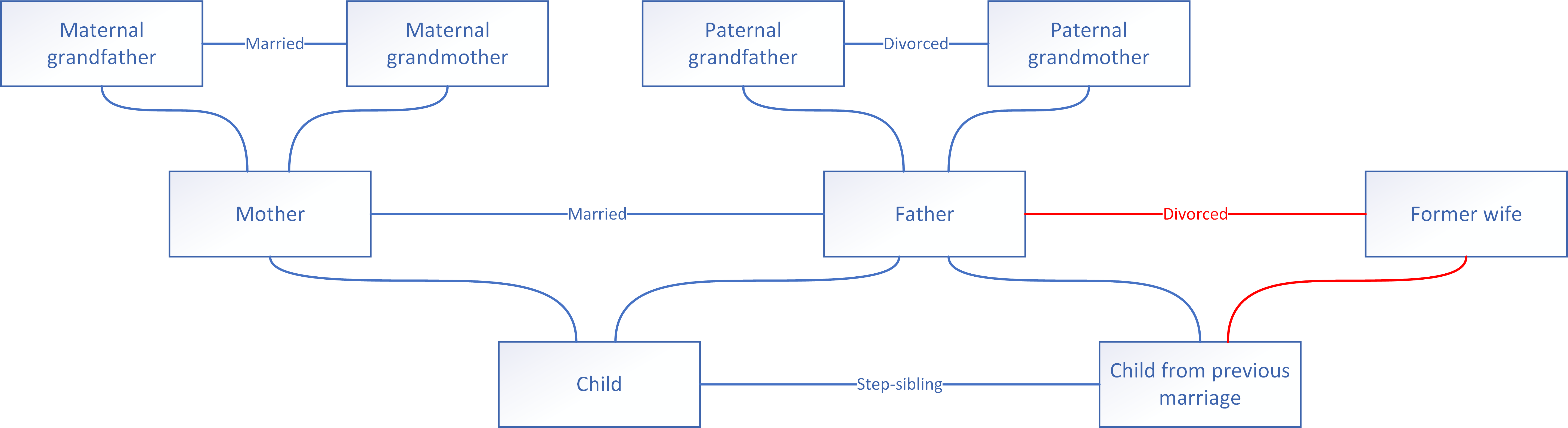
A walk that connects two vertices without any repetition in either the edges or the vertices is called a path. For example, in Figure 1, the maternal grandmother vertex connects to the child vertex through the path consisting of the parent-child edge to the mother vertex, the mother vertex and the parent-child edge from there to the child vertex. This is also the shortest path between the two vertices, shorter than e.g. paths via the father and former wife vertices.

Graph measures

The distance between two vertices is the number of edges in the shortest path between them. In a family tree, the distance between parents and children is always 1 and the distance between grandparents and grandchildren is 2 (Table 3).

Table 3. Distances in the family tree graph

	Maternal grandmother	Maternal grandfather	Paternal grandmother	Paternal grandfather	Mother	Father	Former wife	Child	Child from former marriage
Maternal grandmother	×	1	3	3	1	2	3	2	3
Maternal grandfather	1	×	3	3	1	2	3	2	3
Paternal grandmother	3	3	×	1	2	1	2	2	2
Paternal grandfather	3	3	1	×	2	1	2	2	2
Mother	1	1	2	2	×	1	2	1	2
Father	2	2	1	1	1	×	1	1	1
Former wife	3	3	2	2	2	1	×	2	1
Child	2	2	2	2	1	1	2	×	1
Child from previous marriage	3	3	2	2	2	1	1	1	×

The distance is the basis for a range of measures, starting with eccentricity: the greatest distance between a vertex and any other vertex in a graph. Eccentricity is a good indication of the centrality of a vertex in a graph. It is also an indication of the size of the graph: the radius of a graph is the smallest eccentricity of any vertex in the graph and the diameter of a graph is the greatest eccentricity of any vertex in the graph. The vertices with an eccentricity equal to the radius form the center of the graph, while the vertices with an eccentricity equal to the diameter form the periphery (Table 4).

Table 4. Distances in the metro graph

	A	B	C	D	E	F	G	H	I	J	K	L	M	N	Eccentricity	Closeness
A	×	1	2	3	4	5	6	7	6	5	4	4	5	6	7	0,31
B	1	×	1	2	3	4	5	6	5	4	3	3	4	5	6	0,38
C	2	1	×	1	2	3	4	5	4	3	2	2	3	4	5	0,50
D	3	2	1	×	1	2	3	4	3	2	1	1	2	3	4	0,72
E	4	3	2	1	×	1	2	5	4	3	2	2	3	4	5	0,59
F	5	4	3	2	1	×	1	6	5	4	3	3	4	5	6	0,50
G	6	5	4	3	2	1	×	7	6	5	4	4	5	6	7	0,41
H	7	6	5	4	5	6	7	×	1	2	3	5	6	7	7	0,43
I	6	5	4	3	4	5	6	1	×	1	2	4	5	6	6	0,54
J	5	4	3	2	3	4	5	2	1	×	1	3	4	5	5	0,65
K	4	3	2	1	2	3	4	3	2	1	×	2	3	4	4	0,72
L	4	3	2	1	2	3	4	5	4	3	2	×	1	2	5	0,59
M	5	4	3	2	3	4	5	6	5	4	3	1	×	1	6	0,46
N	6	5	4	3	4	5	6	7	6	5	4	2	1	×	7	0,36

In the example of the metro map, these measures suggest that vertices D and K are the center, and vertices A, G, H and N the periphery (Figure 6). In between the two are vertices with eccentricities of 5 and 6. These groups agree with intuitive interpretations of the metro map. You may also choose to form the center out of vertices with an eccentricity of 4 and 5 or the periphery out of vertices with an eccentricity of 6 and 7. Using ranges of values also agrees with intuitive interpretations and can be useful with large graphs.

Figure 6. The center and the periphery of the metro graph

In addition to eccentricity, you can use the closeness of a vertex: its inverse mean distance to all other vertices in the graph, calculated by dividing the number of all other vertices (the order of the graph minus one) by the sum of distances to these vertices. The higher the value of closeness, the more central the position of a vertex (Table 4). In the example of the metro map, closeness and eccentricity agree that vertices D and K are the most central. As for the rest of the vertices, the closeness values offer more variation than eccentricity and thus a more refined basis for grouping them.

Directed graphs

Many relations are directed by their precedence in time, in relation to movement or through another dependence, as in the relation between parent and child. These can be represented in directed graphs (digraphs), where things are represented by nodes (a synonym of vertex, which we will use to indicate that we are dealing with a digraph) and relations by arcs (i.e. directed edges). Due to directedness, some things are slightly different from undirected graphs:

• A node has an in- and an out-degree, measured respectively by the number of incoming and out outgoing arcs. A node with an in-degree of 0 is called a source. Source nodes are the starting points of processes. A node with an out-degree of 0 is called a terminal (or sink) and represents an endpoint in a process.
• A walk is directed: it consists of arcs with the same direction.
• A path is similarly directed (dipath): This obviously affects connectivity: a digraph is strongly connected if there is a dipath that connects every pair of nodes or weakly connected if the undirected underlying graph obtained by replacing all arcs with edges in connected.

Graphs that contain both edges and arcs are called mixed and are to be avoided in the context of this book. In the subjects discussed here, either the direction does not matter (as with most doors in a building) or is strictly defined by time or dependence (as in the transition from one task to another in a process). It may be tempting to add bidirectional arcs to process diagrams but these, too, should be avoided because they merely obfuscate the process, e.g. obscure feedback.

Graph operations

The changes you apply to a graph include:

• Edge contraction: the replacement of an edge and two vertices incident to it with a single vertex
• Edge subdivision: the replacement of an edge with a vertex and connection of the new vertex with new edges to the ends of the original vertices

• Vertex identification: replacement of any two vertices with a single vertex incident to all edges previously incident to either of the original vertices
• Vertex splitting: the replacement of a vertex with two adjacent vertices and of each edge incident to the original vertex with an edge incident to either new vertex (but not to both)

In all transformations of a graph, it is advisable to think in terms of these operations to ensure consistency and avoid omissions, such as forgetting to connect a new node to the existing ones when refining a process diagram. They help connect the previous state of the graph to the new one and to meaning of the changes you want to implement. In particular, the transition from process to information diagram involves changes that benefit from considering them as graph operations.