5.6: Sorting and Filtering

Last updated
Save as PDF

Page ID: 14322

\( \newcommand{\vecs}[1]{\overset { \scriptstyle \rightharpoonup} {\mathbf{#1}} } \) \( \newcommand{\vecd}[1]{\overset{-\!-\!\rightharpoonup}{\vphantom{a}\smash {#1}}} \)\(\newcommand{\id}{\mathrm{id}}\) \( \newcommand{\Span}{\mathrm{span}}\) \( \newcommand{\kernel}{\mathrm{null}\,}\) \( \newcommand{\range}{\mathrm{range}\,}\) \( \newcommand{\RealPart}{\mathrm{Re}}\) \( \newcommand{\ImaginaryPart}{\mathrm{Im}}\) \( \newcommand{\Argument}{\mathrm{Arg}}\) \( \newcommand{\norm}[1]{\| #1 \|}\) \( \newcommand{\inner}[2]{\langle #1, #2 \rangle}\) \( \newcommand{\Span}{\mathrm{span}}\) \(\newcommand{\id}{\mathrm{id}}\) \( \newcommand{\Span}{\mathrm{span}}\) \( \newcommand{\kernel}{\mathrm{null}\,}\) \( \newcommand{\range}{\mathrm{range}\,}\) \( \newcommand{\RealPart}{\mathrm{Re}}\) \( \newcommand{\ImaginaryPart}{\mathrm{Im}}\) \( \newcommand{\Argument}{\mathrm{Arg}}\) \( \newcommand{\norm}[1]{\| #1 \|}\) \( \newcommand{\inner}[2]{\langle #1, #2 \rangle}\) \( \newcommand{\Span}{\mathrm{span}}\)\(\newcommand{\AA}{\unicode[.8,0]{x212B}}\)

Worksheets can have large amounts of data, and it can be overwhelming if it is not sorted correctly. Arranging data in a specified order is called sorting. Rows can be sorted in either ascending (low to high) or descending (high to low) order. Ascending order can also be considered alphabetic order if the data is text or chronological order if the data is dates or times.

Before data can be sorted, Excel needs to know the exact range of cells that is to be sorted. Excel will select areas of related data as long as there are no blank rows or columns in the data range. Blank rows and columns define the outer limits of the data range. To ensure that the correct data is selected, highlight the range before starting the sort.

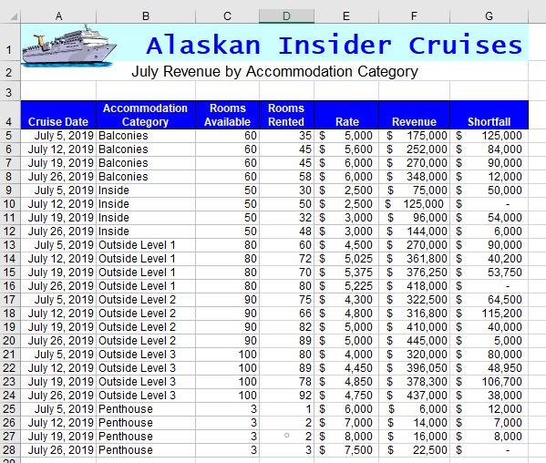
As Excel determines the defined range of data to be sorted, Excel also determines if field names exist. Users should format the first row of the data range with unique formatting Often, just making the labels bold will help Excel identify the field names. Identifying the field names will prevent Excel from including these fields in the records to be sorted. The field names become the sort keys needed for multiple column sorts. In the image below, the possible sort keys are: Cruise Date, Accommodation Category, Rooms Available, Rooms Rented, Rate, Revenue and Shortfall.

The data range above is already sorted in ascending order by the Accommodation Category key field. A single column sort is quite easy. Simply click any cell in the column that represents the key sort. In the above example, any cell from B4 to B28 would be acceptable. Then, click the the A-Z option in the Sort & Filter group of the Data tab. The entire row is sorted because each row is a record that should stay grouped together. Be careful NOT to select a single column of data or the records may not be kept together. Excel will warn the user with a warning message. If the user chooses to Continue with the current selection, only the data in the column with change their order, while the data in the other columns remain unchanged. This will most likely destroy the integrity of the data.

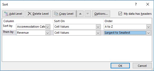
Advanced sorting involves multiple key fields from multiple columns. A multi-level sort can be set up by clicking the Sort button from Sort & Filter group from the Data tab (or the Sort & Filter button from the Editing group of the Home tab and choose Custom Sort) to open the Sort dialog window. The first sort criteria, also known as the primary sort, was previously defined to sort by Accommodation Category in ascending order.

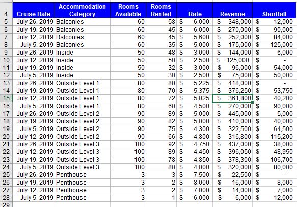
To add a second level, also known as a secondary sort, click the Add Level button. After entering additional sort criteria, additional levels can be added. As shown in the graphic to the right, secondary criteria has been added to sort in descending order by Revenue. The data in column B will not appear to change, but the records will reorder. Compare the results below with the table above.

An Excel filter, also known as an AutoFilter, is used to display only the data that meet specific criteria. Data that does not meet the criteria is hidden from view. Excel’s basic filter functionality allows users to filter rows by value, by format and by criteria. Filters can reduce a large, complex worksheet of data into meaningful information. With filtering, you can control not only what you want to see, but what you want to exclude. Users can filter based on choices they make from a list, or they can create specific filters to focus on exactly the data that they want to see.

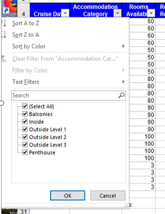
Clicking the filter button from the Data tab will add drop-down arrows to the column headers in a range of data. Clicking a drop-down arrow provides sorting and filtering options, like filter by color or text filters. A simple AutoFilter will be signified by the clearing of check boxes of the data that should be hidden. After applying a filter, a user can copy, edit, chart or print only visible rows without rearranging the entire list. Like sorting, filters can be applied to multiple columns to further reduce the results that are displayed.

A column that has been filtered will have its drop-down arrow icon switch from an upside-down triangle to a filter icon, as shown highlighted in yellow below. Only the cruises from the Penthouse accommodation category will be displayed after clearing all check boxes except the Penthouse category.

Applied Filter2 — Applied Filter example

To remove a single filter, click the filter icon in the row header and choose Clear Filter from…. To clear all filters quickly, choose the Clear button from the Data tab on the ribbon or to remove filtering functionality, re-click the Filter icon from the Sort & Filter group. For more advanced users there are many more ways to utilize filters in Excel, such as Custom Filters and Advanced Filters. Nonetheless, a lot can be accomplished with the basic AutoFilter feature.