5.7: Conditional Formatting

Last updated
Save as PDF

Page ID: 14323

$ \newcommand{\vecs}[1]{\overset { \scriptstyle \rightharpoonup} {\mathbf{#1}} } $ $ \newcommand{\vecd}[1]{\overset{-\!-\!\rightharpoonup}{\vphantom{a}\smash {#1}}} $$\newcommand{\id}{\mathrm{id}}$ $ \newcommand{\Span}{\mathrm{span}}$ $ \newcommand{\kernel}{\mathrm{null}\,}$ $ \newcommand{\range}{\mathrm{range}\,}$ $ \newcommand{\RealPart}{\mathrm{Re}}$ $ \newcommand{\ImaginaryPart}{\mathrm{Im}}$ $ \newcommand{\Argument}{\mathrm{Arg}}$ $ \newcommand{\norm}[1]{\| #1 \|}$ $ \newcommand{\inner}[2]{\langle #1, #2 \rangle}$ $ \newcommand{\Span}{\mathrm{span}}$ $\newcommand{\id}{\mathrm{id}}$ $ \newcommand{\Span}{\mathrm{span}}$ $ \newcommand{\kernel}{\mathrm{null}\,}$ $ \newcommand{\range}{\mathrm{range}\,}$ $ \newcommand{\RealPart}{\mathrm{Re}}$ $ \newcommand{\ImaginaryPart}{\mathrm{Im}}$ $ \newcommand{\Argument}{\mathrm{Arg}}$ $ \newcommand{\norm}[1]{\| #1 \|}$ $ \newcommand{\inner}[2]{\langle #1, #2 \rangle}$ $ \newcommand{\Span}{\mathrm{span}}$$\newcommand{\AA}{\unicode[.8,0]{x212B}}$

Using spreadsheet functionality to enhance critical thinking is a primary reason that Excel is so popular among business professionals. Decision-making is made easier when users can quickly spot trends, identify variances, and be alerted when certain criteria is met. Excel’s conditional formatting feature is a really powerful tool when it comes to applying different formats to data that meets certain conditions. Conditional formatting is one of the most simple yet powerful features in Excel by applying user-specific formats to a cell/cells when user-specific conditions (rules) are met. Not only does it make a spreadsheet look awesome, but it also helps make sense of the data.

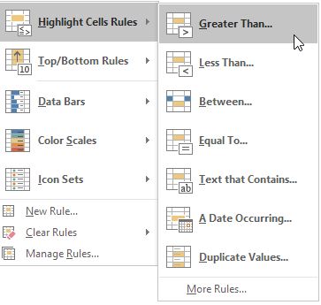
Clicking the Conditional Formatting button on the Home tab of the ribbon offers several options to define the condition criteria (rules), and several formatting options to display the data in meaningful ways. To choose formats that are applied to a cell(s) when a condition is met, select a range of cells, then click the Conditional Formatting button to display a menu of rules. Clicking a rule will expand an additional menu.

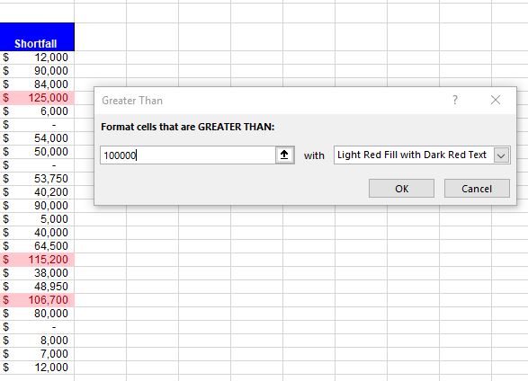
For example to identify which cruise accommodation categories provide the most significant revenue shortfall, utilizing a highlighting rule that formats cells that are greater than $100,000 would be a very practical conditional formatting rule that could provide some strategic information. Selecting the range of G5:G28 and applying the Greater Than rule, will create eye-catching formatting. The data in the first field can either be a cell reference or a static value, as shown below.

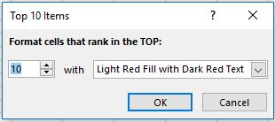
Numerous rule types exist beyond the preset comparison operator menu choices. Rules can identify cells that contain certain text or before/after a certain date, or even highlight duplicate data. Top/Bottom Rules can reveal the top or bottom 10 records in a certain column. The quantity can be modified from the top/bottom 10 to a user-specific number.

Custom rules can be defined by choosing More Rules… from the Highlight Cells Rules menu, which opens the New Formatting Rule window. Choosing alternative Rule Types will modify the functionality available in this window.

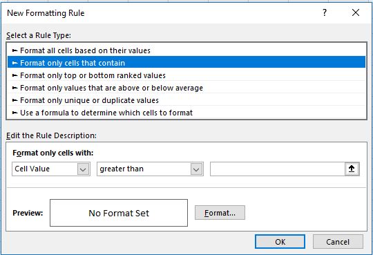
After defining the rule criterion, custom formats can be selected by clicking the Format button. The Format Cells window opens to allow custom Number, Font, Border or Fill formatting.

Icon sets menu

To enforce more complex rules, multiple conditional formatting rules can be applied to the same data. However too many colors can sometimes be distracting, and should be used sparingly. Therefore, Excel offers more formatting choices than just color fills. Data bars, color scales and icon sets can also be used to emphasize data that meets certain conditions.

The icon sets work great when color is not effective, such as when printing to black & white laser printers. Icons are even more noticeable than colors because of their unique look and sparing use. Icon sets will help visually represent the data with directional arrows, shapes, indicators, ratings, and other objects. For icons in sets of three, Excel will assign icons by dividing values into thirds – the first icon is assigned to the top one third of values, the second icon is assigned to the second third of values, and the third icon is assigned to the lowest one third of values. The values are adjusted for four and five-icon sets. Conditional formatting’s flexibility is extensive, but perhaps even more impressive is that, like formulas, conditional formatting rules are volatile. As the data changes, the conditional formatting dynamically adjusts to evaluate the new data against the existing conditional rules.