1.8: Module 7 - Drawings

Introduction

This module looks at creating engineering drawings from a three-dimensional model. Engineering drawings are essentially a communication tool. They are typically used by the designer to communicate with:

1. other designers,
2. machinists,
3. quality technicians, and
4. supply chain associates.

Projecting a three-dimensional object on to two dimensions presents its own challenges. Multiple views of the three-dimensional entity must be created in order to supply complete information in a two-dimensional medium. This two-dimensional medium in this case is the computer screen. However, the drawing space is chosen according to the size of the paper it will eventually be printed on. Paper sizes are classified as American Society of Mechanical Engineers (ASME) A – E, with A being the smallest paper size and E being the largest paper size. Other classifications such as Organisation Internationale de Normalisation (ISO) A0 – A4 can also be used, with A0 being the largest paper size, and A4 being the smallest paper size).

Two-Dimensional Views of Three-Dimensional Objects

The two primary ways to represent a three-dimensional object in two dimensions are: Orthogonal Views and Auxiliary Views. However, three-dimensional objects can also be rendered in a way to give them some sense of depth. This happens in real time in the Autodesk Fusion 360 environment. To translate this three-dimensional rendering on to a two-dimensional drawing, a technique called the isometric view, as shown in Figure \(\PageIndex{1}\), is used. Note that for a highly symmetrical object with no angled surfaces, the isometric view works well to convey all the information about the dimensions of the object.

Figure \(\PageIndex{1}\): Isometric view (left) of a three-dimensional rendering (right) of the square base plate covered in Module 5.

Orthogonal View

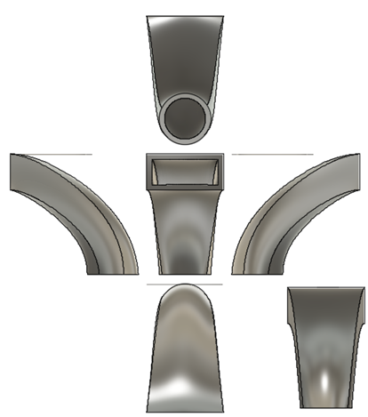
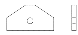
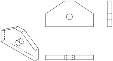
To perceive orthogonal views, imagine the object being freely suspended inside a glass box. To look at the object you could place it such that you are looking straight at it in one of six orientations: top/bottom, front/back, and left/right side. All of these six views have been shown in Figure \(\PageIndex{2}\).

Figure \(\PageIndex{2}\): Orthogonal views for a Heating Ventilation and Air Conditioning (HVAC) duct.

Auxiliary View

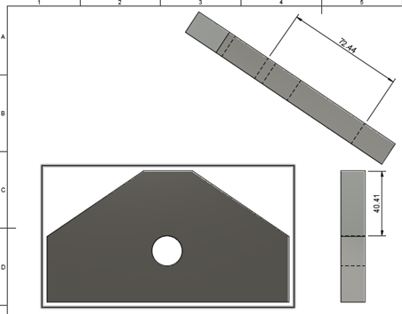
Any view obtained by a projection on a plane other than the horizontal (H), frontal (F) and profile (P) is an auxiliary view.

For a three-dimensional object with angled surfaces that cannot be projected accurately on the planes mentioned above, there need to be auxiliary planes that will accomplish that. In Figure \(\PageIndex{3}\), when the orthogonal view of the bracket is created, the length of the angled side is measured at 40.41 millimeters (mm). However, this measurement is inaccurate. In order to get the accurate measurement on the drawing, it must be measured on an auxiliary plane parallel to the angled edge.

Figure \(\PageIndex{3}\): Projection on Auxiliary Planes.

Dimensioning

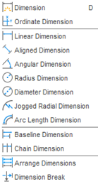
As noted in the previous sections, accurate dimensions are an essential component of the engineering drawing. There are several strategies to place dimensions in an engineering drawing. Dimensions can be placed on the X or Y axis, can be continuous or broken down, or can be placed such that they align with the shape being labeled. Text can be added to engineering drawings in order to add any specific notes or instructions. Like dimensions, text can be customized to be placed in different orientations, fonts, and alignments. All the available options for dimensioning in Autodesk Fusion 360 are shown in Figure \(\PageIndex{4}\).

Figure \(\PageIndex{4}\): Dimensioning options available in the drawing mode of Autodesk Fusion 360.

Dimension

The Dimension option allows for creating linear, aligned, angular, radius, and diameter dimensions for a drawing entity, such as a line, arc, circle or points. This option automatically latches on to the type of the entity. (See Figure \(\PageIndex{5}\))

Figure \(\PageIndex{5}\): Icon for the Dimension option.

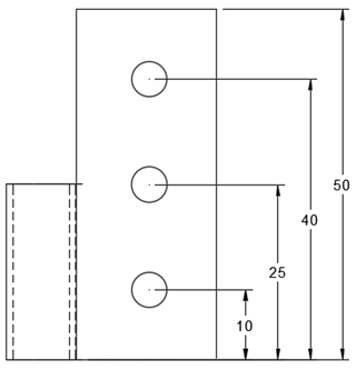
Ordinate Dimension

The Ordinate Dimension option allows for creating dimensions references from an origin defined by the user. (See Figure \(\PageIndex{6}\).)

Figure \(\PageIndex{6}\): Icon for the Ordinate Dimension option.

This option is especially useful if the component in the drawing has multiple dimensions along the X or Y axis that will be useful during manufacturing the component. For example the hinge shown in Figure \(\PageIndex{7}\), has the center points of all the holes on the plate of the hinge dimensioned using ordinate dimensions. If the hole were to be drilled out using a drill press, the drill operator would not need to do any additional calculations to see how far the drill head or the workpiece must be moved from the base of the hinge plate to accurately drill the holes.

Figure \(\PageIndex{7}\): An example of Ordinate Dimensioning used for a hinge base plate.

Linear Dimension:

The Linear Dimension option allows for measuring the horizontal or vertical distance between two points or an edge. (See Figure \(\PageIndex{8}\).)

Figure \(\PageIndex{8}\): Icon for the Linear Dimension option.

Aligned Dimension

The Aligned dimension option allows for measuring the distance between two points that may not be either vertical or horizontal. (See Figure \(\PageIndex{9}\).)

Figure \(\PageIndex{9}\): Icon for the Aligned Dimension option.

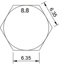
Figure \(\PageIndex{10}\) shows the hexagonal head of an M7 bolt. Since it is a regular hexagon, all its sides are the same length. To label the length of a horizontal edge of the hexagon, linear dimension can be used. However, if the user chooses to dimension one of the non-horizontal edges, then an aligned dimension should be used.

Figure \(\PageIndex{10}\): Linear and Aligned Dimension used for the hexagonal head of an M7 bolt.

Radius Dimension

The Radius dimension option allows for dimensioning a circular entity using its radius. (See Figure \(\PageIndex{11}\).)

Figure \(\PageIndex{11}\): Icon for Radius Dimension option.

Diameter Dimension

The diameter dimension option allows for dimensioning a circular entity using its diameter. (See Figure \(\PageIndex{12}\).)

Figure \(\PageIndex{12}\): Icon for the Diameter Dimension option.

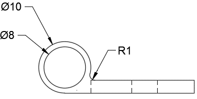
Consider the front view of the hinge base plate as shown in Figure \(\PageIndex{13}\). The inner and outer diameter of the hole where the pin is supposed to sit is dimensioned with the diameter annotation ϕ (Greek alphabet letter phi). The fillet radius is dimensioned with radius annotation R.

Figure \(\PageIndex{13}\): Circular features on the front view of a hinge base plate dimension dimensioned using Radius and Diameter Dimension.

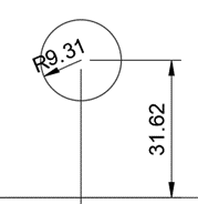
Jogged Radial Dimension

The Jogged Radial dimension allows for dimensioning a circular component with dimension running from the center of the circular entity to its edge. It can also be jogged to a more convenient place within the circular entity for increased legibility. (See Figures \(\PageIndex{14}\) and \(\PageIndex{15}\).)

Figure \(\PageIndex{14}\): Icon for the Jogged Radial Dimension option.

Figure \(\PageIndex{15}\): Example of a jogged radial dimension placed away from the linear dimension.

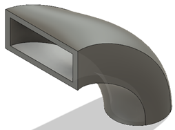
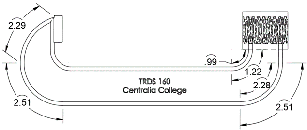
Arc Length Dimension

The Arc Length dimension allows for dimensioning the length of an arc. (See Figure \(\PageIndex{16}\).)

Figure \(\PageIndex{16}\): Icon for the Arc Length option.

Consider the C-Clamp of a vice shown in Figure \(\PageIndex{17}\). There are several arcs used in solid model. They can be labeled in the drawing using the arc length option.

Figure \(\PageIndex{17}\): Arc Length Dimension option used to label the arc lengths of a C clamp.

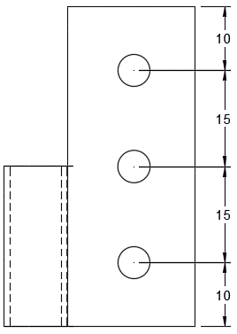
Baseline Dimension

The Baseline Dimension option allows the user to use an existing linear dimension as a base point to create a new linear dimension. (See Figures \(\PageIndex{18}\) and \(\PageIndex{19}\).)

Figure \(\PageIndex{18}\): Icon for the Baseline Dimension option.

The holes of the hinge base plate shown in Figure \(\PageIndex{19}\) have been dimensioned using baseline dimension option. The base dimension used is the distance from the base to center of the first hole, i.e. 10 mm.

Figure \(\PageIndex{19}\): Baseline Dimension option used to label the distances of the holes from the base of the hinge plate.

Chain Dimension

Allows the user to use an existing linear dimension to create a new linear chain dimension.

Figure \(\PageIndex{20}\): Icon for the Chain Dimension option.

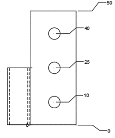
The holes of the hinge base plate shown in Figure \(\PageIndex{21}\) have been dimensioned using chain dimension option. The base dimension used is the distance from the base to center of the first hole, i.e. 10 mm.

Figure \(\PageIndex{21}\): Chain Dimension option used to label the distances of the holes from the base of the hinge plate.

Geometric Dimensioning and Tolerancing

Geometric Dimensioning and Tolerancing (GD&T) is used in the industry to communicate dimensioning specifications using a standard set of symbols. These symbols are reviewed and prescribed by ASME in their Y14.5-2018 standard and internationally by ISO in their 1101:2017 standard. Fusion 360 incorporates most of these symbols under its symbols option as shown in Figure \(\PageIndex{22}\).

Figure \(\PageIndex{22}\): Icons for the GD&T options available in the drawing mode of Autodesk Fusion 360.

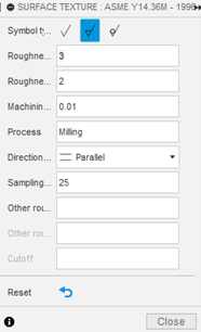
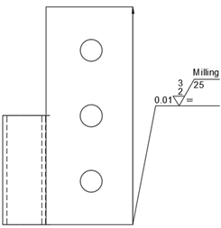
Surface Finish

The surface texture symbol allows for the designer to specify the machining operations, minimum and maximum surface roughness, and the amount of material that is to be removed from a surface. The surface finish symbol is shown in Figure \(\PageIndex{23}\). The dialog box for inputting the surface finish parameters is shown in Figure \(\PageIndex{24}\). To apply the surface finish symbol to a solid model imported into a drawing, select an edge or feature to which the symbol has to be applied. In Figure \(\PageIndex{24}\), the base plate of the hinge has a surface finish symbol applied to it. The operation specified is milling, the maximum and the minimum surface roughness is 3 and 2 micrometers, machining allowance is 0.01 mm, and the sampling length is 25 mm. The symbol is generated and applied as per ASME standard.

Figure \(\PageIndex{23}\): Icon for the Surface Finish option.

Figure \(\PageIndex{24}\): Surface Finish Symbols as applied to the base plate of the hinge.

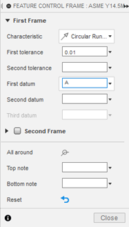
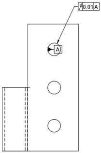
Feature Control Frame

The feature control frame allows the user to call out a specific feature of the solid model in a drawing and add symbols that signify the tolerances for it. The icon for feature control frame is shown in Figure \(\PageIndex{25}\). The dialog box for inputting the feature control parameters is shown in Figure \(\PageIndex{26}\). To apply the surface finish symbol to a solid model imported into a drawing, select a feature to which the symbol has to be applied. In Figure \(\PageIndex{26}\), a hole on the base plate of the hinge has a control frame symbol applied to it. The tolerance specified is circular runout, which cannot exceed 0.01 mm around the datum A, which is the axis of the hole feature. The symbol is generated and applied as per ASME standard.

Figure \(\PageIndex{25}\): Icon for the Feature Control Frame.

Figure \(\PageIndex{26}\): Feature Control Frame as applied to the base plate of the hinge.

Other symbols

In addition to surface texture and feature control, Fusion 360 also allows for other symbols associated with GD&T, such as datum identifiers, taper and slope identifiers and welding symbols. These symbols are also reviewed and prescribed by ASME in the United States and internationally by ISO.

Create a drawing from a Solid model

First a sketch of the solid model will have to be created. Once the sketch has been completed, the solid model will be extruded and a hole feature would be added. Then, the solid model will be imported into a drawing.

Module 7 step-by-step videos:

Part 1 - https://youtu.be/QyLWUj-JMSs - Transcript is available on YouTube.

Part 2 - https://youtu.be/0pvv_LE_wj8 - Transcript is available on YouTube.

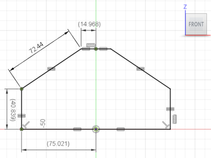
Step 1 - Create the sketch

Start a new sketch file. Create and constrain the sketch as shown in the Figure \(\PageIndex{27}\). It is a six-sided polygon with base length of 150.042 mm, sides of 40.839 mm, angled sides of 72.44 mm, and top edge 29.936 mm. Make sure to finish the sketch after completion.

Figure \(\PageIndex{27}\): Sketch of the solid model to be created.

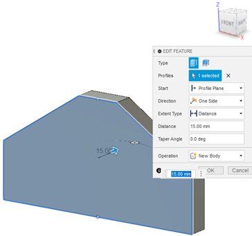
Step 2 - Extrude the sketch

Extrude the sketch to a thickness of 15 mm as shown in the figure \(\PageIndex{28}\).

Figure \(\PageIndex{28}\): Extruded sketch.

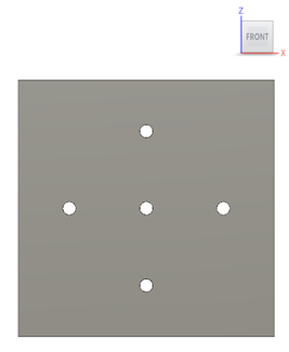
Step 3 - Sketch a circle on the face of the solid model

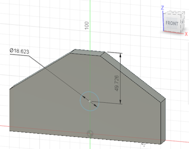
Sketch a hole on the face of the solid model just created. Use the dimensions and the centerline to create the circle. The center of the circle of diameter 18.623 mm is on the centerline and is 49.726 mm away from the top edge as shown in Figure \(\PageIndex{29}\).

Figure \(\PageIndex{29}\): Sketch a circle on the face of the solid model.

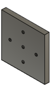
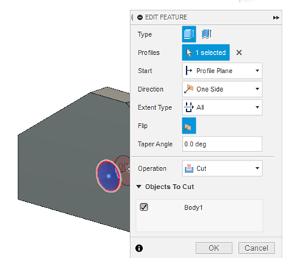
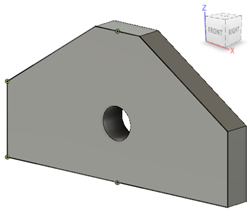
Step 4 - Extrude cut the circle to form a hole

Extrude cut the circle sketch to form a through hole as shown in \(\PageIndex{30}\). This is a one sided through hole. The finished model will look like the one in figure \(\PageIndex{31}\).

Figure \(\PageIndex{30}\): Extrude cut hole in solid model.

Figure \(\PageIndex{31}\): Finished solid model.

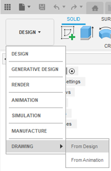
Step 5 - Import the model into the drawing

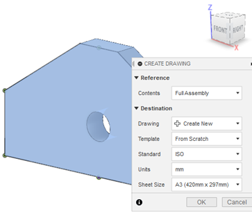
While this solid model tab is still open, from the top left corner of the screen, click on “Design”. From the drop down menu, select Drawing > From Design as shown in Figure \(\PageIndex{32}\). The solid model will turn light blue and a dialog box for the setting for the drawing will open up.

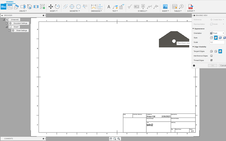
Once you click Ok on the dialog box, the drawing tab opens up as shown in Figure \(\PageIndex{33}\). Select an appropriate sheet size and scale. For this particular model, an A3 sheet size and a scale of 1:2.

Figure \(\PageIndex{32}\): Importing a solid model into a drawing.

Figure \(\PageIndex{33}\): Drawing tab with the imported solid model.

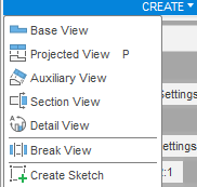
Step 6 - Create additional views

Under the Create tab, additional views of the drawing can be created. As discussed earlier in this module, it is often insufficient to convey all the information involved in manufacturing the solid model from a 3D CAD file using just one view. All the options for adding these views are shown in \(\PageIndex{34}\).

Figure \(\PageIndex{34}\): Additional views that can be added in the drawing.

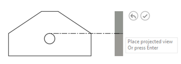
Projected view

This option creates orthogonal and isometric views from the base view. A side view for this solid model can be added as shown in figure \(\PageIndex{35}\).

Figure \(\PageIndex{35}\): Adding a projected view for the solid model.

Similarly, a bottom view and an isometric view can be added. The resulting drawing should look like figure \(\PageIndex{36}\).

Figure \(\PageIndex{36}\): Base view and isometric view added using projected view.

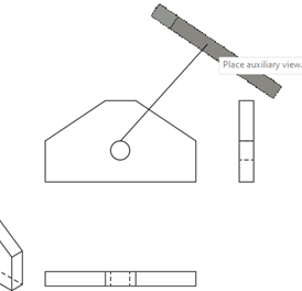
Auxiliary View

Add an auxiliary view as shown in \(\PageIndex{37}\). As discussed earlier in this module, auxiliary views are necessary for displaying the accurate dimensions of an angled feature on a solid model.

Figure \(\PageIndex{37}\): Adding an auxiliary view.

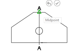
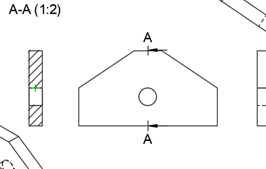
Section View

Select section view and place the sectioning datum as shown in figure \(\PageIndex{38}\). Think of this datum as a knife that will slice this solid model in half. Once this datum, AA (scale 1:2), is finalized, place this section view on the left side of the base view. The hatching represents the solid sections of the solid model and the non- hatched part represents the hole in the center of this solid model.

Figure \(\PageIndex{38}\): Adding a section view.

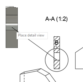
Detail View

In order to create a more detailed view of the hole, select the section view and select the section view as the base view as shown in figure \(\PageIndex{39}\). A scale of 1:1 is appropriate for this.

Figure \(\PageIndex{39}\): Adding a detail view.

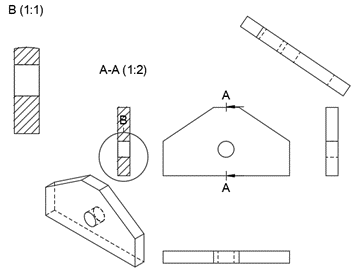
The drawing sheet at this point should look like the figure \(\PageIndex{40}\).

Figure \(\PageIndex{40}\): Drawing file after adding all the views.

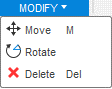
Modifying the drawing

Should you choose to delete or move or rotate any of the views on the drawing sheet, the Modify drop down menu allows for this. All the options available are shown in figure \(\PageIndex{41}\).

Figure \(\PageIndex{41}\): Modify options available to modify the views on the drawing sheet.

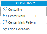
Geometry Call Outs

Should you choose to call out the geometry features on any of the views on the drawing sheet, the Geometry drop down menu allows for this. All the options available are shown in figure \(\PageIndex{42}\).

Figure \(\PageIndex{42}\): Geometry call out options.

Add Dimensions to the Drawing

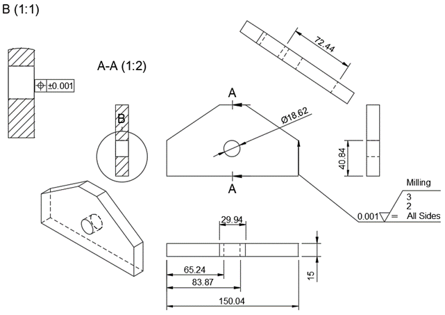
As discussed in the previous sections in this module, add the following dimensions and symbols to the drawing as shown in figure \(\PageIndex{43}\).

Figure \(\PageIndex{43}\): Completed drawing with all the dimensions and symbols.

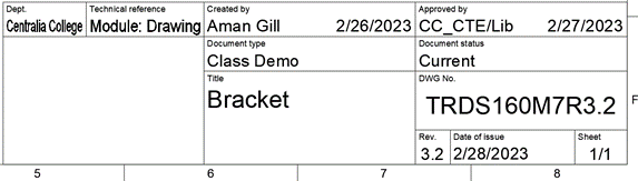
Edit the Drawing Description

Double click the drawing description table and edit the description as appropriate. An example of this is shown in figure \(\PageIndex{44}\).

Figure \(\PageIndex{44}\): Drawing description.

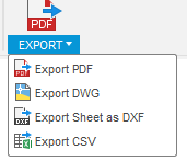
Save and/or Export the Drawing

The drawing that has just been completed should now be saved. It can also be exported to a PDF file format using the export option as shown in figure \(\PageIndex{45}\).

Figure \(\PageIndex{45}\): Export options to export drawing from an Autodesk Fusion 360 file to an Adobe Acrobat file (PDF).