4.3: Software Usage Assignment
- Page ID
- 13029
\( \newcommand{\vecs}[1]{\overset { \scriptstyle \rightharpoonup} {\mathbf{#1}} } \)
\( \newcommand{\vecd}[1]{\overset{-\!-\!\rightharpoonup}{\vphantom{a}\smash {#1}}} \)
\( \newcommand{\id}{\mathrm{id}}\) \( \newcommand{\Span}{\mathrm{span}}\)
( \newcommand{\kernel}{\mathrm{null}\,}\) \( \newcommand{\range}{\mathrm{range}\,}\)
\( \newcommand{\RealPart}{\mathrm{Re}}\) \( \newcommand{\ImaginaryPart}{\mathrm{Im}}\)
\( \newcommand{\Argument}{\mathrm{Arg}}\) \( \newcommand{\norm}[1]{\| #1 \|}\)
\( \newcommand{\inner}[2]{\langle #1, #2 \rangle}\)
\( \newcommand{\Span}{\mathrm{span}}\)
\( \newcommand{\id}{\mathrm{id}}\)
\( \newcommand{\Span}{\mathrm{span}}\)
\( \newcommand{\kernel}{\mathrm{null}\,}\)
\( \newcommand{\range}{\mathrm{range}\,}\)
\( \newcommand{\RealPart}{\mathrm{Re}}\)
\( \newcommand{\ImaginaryPart}{\mathrm{Im}}\)
\( \newcommand{\Argument}{\mathrm{Arg}}\)
\( \newcommand{\norm}[1]{\| #1 \|}\)
\( \newcommand{\inner}[2]{\langle #1, #2 \rangle}\)
\( \newcommand{\Span}{\mathrm{span}}\) \( \newcommand{\AA}{\unicode[.8,0]{x212B}}\)
\( \newcommand{\vectorA}[1]{\vec{#1}} % arrow\)
\( \newcommand{\vectorAt}[1]{\vec{\text{#1}}} % arrow\)
\( \newcommand{\vectorB}[1]{\overset { \scriptstyle \rightharpoonup} {\mathbf{#1}} } \)
\( \newcommand{\vectorC}[1]{\textbf{#1}} \)
\( \newcommand{\vectorD}[1]{\overrightarrow{#1}} \)
\( \newcommand{\vectorDt}[1]{\overrightarrow{\text{#1}}} \)
\( \newcommand{\vectE}[1]{\overset{-\!-\!\rightharpoonup}{\vphantom{a}\smash{\mathbf {#1}}}} \)
\( \newcommand{\vecs}[1]{\overset { \scriptstyle \rightharpoonup} {\mathbf{#1}} } \)
\( \newcommand{\vecd}[1]{\overset{-\!-\!\rightharpoonup}{\vphantom{a}\smash {#1}}} \)
\(\newcommand{\avec}{\mathbf a}\) \(\newcommand{\bvec}{\mathbf b}\) \(\newcommand{\cvec}{\mathbf c}\) \(\newcommand{\dvec}{\mathbf d}\) \(\newcommand{\dtil}{\widetilde{\mathbf d}}\) \(\newcommand{\evec}{\mathbf e}\) \(\newcommand{\fvec}{\mathbf f}\) \(\newcommand{\nvec}{\mathbf n}\) \(\newcommand{\pvec}{\mathbf p}\) \(\newcommand{\qvec}{\mathbf q}\) \(\newcommand{\svec}{\mathbf s}\) \(\newcommand{\tvec}{\mathbf t}\) \(\newcommand{\uvec}{\mathbf u}\) \(\newcommand{\vvec}{\mathbf v}\) \(\newcommand{\wvec}{\mathbf w}\) \(\newcommand{\xvec}{\mathbf x}\) \(\newcommand{\yvec}{\mathbf y}\) \(\newcommand{\zvec}{\mathbf z}\) \(\newcommand{\rvec}{\mathbf r}\) \(\newcommand{\mvec}{\mathbf m}\) \(\newcommand{\zerovec}{\mathbf 0}\) \(\newcommand{\onevec}{\mathbf 1}\) \(\newcommand{\real}{\mathbb R}\) \(\newcommand{\twovec}[2]{\left[\begin{array}{r}#1 \\ #2 \end{array}\right]}\) \(\newcommand{\ctwovec}[2]{\left[\begin{array}{c}#1 \\ #2 \end{array}\right]}\) \(\newcommand{\threevec}[3]{\left[\begin{array}{r}#1 \\ #2 \\ #3 \end{array}\right]}\) \(\newcommand{\cthreevec}[3]{\left[\begin{array}{c}#1 \\ #2 \\ #3 \end{array}\right]}\) \(\newcommand{\fourvec}[4]{\left[\begin{array}{r}#1 \\ #2 \\ #3 \\ #4 \end{array}\right]}\) \(\newcommand{\cfourvec}[4]{\left[\begin{array}{c}#1 \\ #2 \\ #3 \\ #4 \end{array}\right]}\) \(\newcommand{\fivevec}[5]{\left[\begin{array}{r}#1 \\ #2 \\ #3 \\ #4 \\ #5 \\ \end{array}\right]}\) \(\newcommand{\cfivevec}[5]{\left[\begin{array}{c}#1 \\ #2 \\ #3 \\ #4 \\ #5 \\ \end{array}\right]}\) \(\newcommand{\mattwo}[4]{\left[\begin{array}{rr}#1 \amp #2 \\ #3 \amp #4 \\ \end{array}\right]}\) \(\newcommand{\laspan}[1]{\text{Span}\{#1\}}\) \(\newcommand{\bcal}{\cal B}\) \(\newcommand{\ccal}{\cal C}\) \(\newcommand{\scal}{\cal S}\) \(\newcommand{\wcal}{\cal W}\) \(\newcommand{\ecal}{\cal E}\) \(\newcommand{\coords}[2]{\left\{#1\right\}_{#2}}\) \(\newcommand{\gray}[1]{\color{gray}{#1}}\) \(\newcommand{\lgray}[1]{\color{lightgray}{#1}}\) \(\newcommand{\rank}{\operatorname{rank}}\) \(\newcommand{\row}{\text{Row}}\) \(\newcommand{\col}{\text{Col}}\) \(\renewcommand{\row}{\text{Row}}\) \(\newcommand{\nul}{\text{Nul}}\) \(\newcommand{\var}{\text{Var}}\) \(\newcommand{\corr}{\text{corr}}\) \(\newcommand{\len}[1]{\left|#1\right|}\) \(\newcommand{\bbar}{\overline{\bvec}}\) \(\newcommand{\bhat}{\widehat{\bvec}}\) \(\newcommand{\bperp}{\bvec^\perp}\) \(\newcommand{\xhat}{\widehat{\xvec}}\) \(\newcommand{\vhat}{\widehat{\vvec}}\) \(\newcommand{\uhat}{\widehat{\uvec}}\) \(\newcommand{\what}{\widehat{\wvec}}\) \(\newcommand{\Sighat}{\widehat{\Sigma}}\) \(\newcommand{\lt}{<}\) \(\newcommand{\gt}{>}\) \(\newcommand{\amp}{&}\) \(\definecolor{fillinmathshade}{gray}{0.9}\)The purpose of this assignment is to:
1. Create column, pie, and bar charts
2. Determine what data to select for which charts
3. Move and Resize Charts
4. Place multiple charts on one page
Preparation: (Review these terms)
- Launcher Button
- Insert a Header
New Terms: (Terms are bolded in the steps in the Assignment below)
- Select data for a column chart. (Step #2, Page 1)
- Create a Cluster Column chart. (Step #3, Pages 1-2)
- Using a new toolbar called Chart Tools. (Step #4, Page 2)
- From Design tools – Add chart elements: Legend. (Step #6, Page 3)
- Change Chart Title to a new title. (Step #7, Page 3)
- Move a chart. (Step # 9, Page 3)
- Selecting the correct data for a Pie Chart. (Step #10, Page 3)
- Create a 3-D Pie Chart. (Step #11, Page 3)
- Exploding a pie slice. (Step #14, Page 4)
- Copy a chart. (Step #16, Page 4)
- Change an existing chart to a different type of chart. (Step #17, Page 4)
- Change the color of the bars of a chart. (Step #18, Page 4)
- Check the Page Orientation. (Step #21, Page 4)
- Adjusting the size of charts. (Step #22, Page 4)
Narrative:
Charts help explain data to those who are not familiar with reading spreadsheets. It is fun and easy to create charts. Using different techniques, charts can have different colors, styles, and layout. (THIS ASSIGNMENT IS WORTH 20 POINTS. THE RUBRIC IS ON PAGE 6)
Software Usage Assignment
1. Open the spreadsheet called SOFTWARE USAGE and save it by the same name.
2. Select data for a column chart. Select range A3 to F7. (Be sure NOT to include row 8)
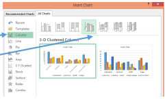
3. Create a Cluster Column Chart.
- Click on the INSERT tab and find the Charts group.
- Click on the Charts launcher button.

- Click on ALL CHARTS.

- Click on Cluster Column
- Click on the fourth example called 3D Cluster

- Click OK
4. Chart Tools Toolbar. After selecting a chart, a new toolbar appears at the top of the screen called Chart Tools with the options of

On the Design portion of the Charts Tools Toolbar, the five groups are:
- Chart Layout
- Chart Styles
- Data
- Type
- Location

On the Format portion of the Charts Tools Toolbar, the five groups are
- Current Selection
- Insert Shapes
- Shape Styles
- WordArt Styles
- Arrange Size
5. Click on the Design tab and look to the left for the Chart Layouts group. Choose Add Chart Elements icon.
The list includes: Axis, Axis Titles, Chart Titles Data Labels, Gridlines and Legends.
6. Add chart elements: Legend. With the Add Chart Element displaying, click on Legend from the drop down menu. From the choices in the drop down menu. choose RIGHT to place the legend on the right side of the chart.
7. Change Chart Title to a new title. Click the “Chart Title” at the top of the graphic chart. A box appears around the “Chart Title”
8. Click in that box and change the title to “Software Usage.”
9. Move a chart. Click on the chart.
- Four white circle should be seen in each of the four corners.
- Place your cursor in the upper left corner of the chart until the mouse becomes a four-headed arrow.
- Click and hold the left mouse and drag the chart so that the top left corner of the chart is in cell A10 and the bottom left corner is in about cell A24. (WARNING: If the chart is pulled too close to the left edge of A10, a red circle displays which will not allow the chart to be placed there. Instead move the chart a bit to the right of cell A10.
- The chart should only be slightly narrower than the data table we started with
Chart 2: Create a Pie Chart
10. Select specific data for Pie Chart. Pie Chart is used to emphasize one data point instead of an entire table. Select A3 to F4
11. Create a Pie Chart. Follow the Steps 3 a-c to INSERT and select ALL CHARTS. Then click Pie Chart. Click on the second example called 3D Pie Chart. Then click OK.
12. The Pie Chart appears and the title of the chart is Middle School (which the name in cell A3)
13. Move the chart to a clear space by clicking on the chart, holding down the left mouse button and dragging it a bit to the right so it is in its own space.
14. Exploding the Pie Slice.
- Click twice on the wedge labeled Foreign Language (it is a gold color). By clicking twice you should see three round white circles on just that slice – on the tip and one on either side of the wedge.
- Holding down the left mouse button, click and drag that wedge toward to the bottom left corner of the chart just a short distance so that it separates itself from the main pie. This is called Exploding the Pie Slice.
15. Move this chart under the column chart. Place the top left edge of the pie chart inside cell A26 and the bottom left on A49.
Chart 3: Create a Bar Chart and Change Colors
16. Copy a Chart. Click on the 3D Cluster Column chart so that the four corners have a white circle on each corner.
- Place the cursor in the upper left corner of the chart, opposite the title, and RIGHT click.
- A short cut menu appears. Choose COPY.
- Move the mouse to the clear area to the right of the other charts. RIGHT click again and this time choose PASTE.
- Remove the Shadow effects by clicking on each of the columns that have the shadow, then from the INSERT tab, Shape Styles Group, click Shape Effects.
- Choose Shadow and then the first choice No Shadow.
17. Change an existing chart to a different type of chart.
- Click in the graph part of the Cluster Column Chart in a white area so that the columns themselves are selected with only the four white circles in each corner.
- Click on INSERT tab, then in the Charts group, click the charts launcher button.
- Click on the tab ALL CHARTS (if it isn’t already selected) and choose Bar Chart.
- Choose the second icon from the Bar Chart called Stacked Bar. The Column Cluster chart changes to the Stacked Bar chart.
18. Change the colors of the chart.
- Click on the white area of the bars of the chart so only four white circles are at each of the corners. (Don’t select just one particular bar.)
- Click on the Design Tab of the Chart Tools and find “Change Colors” in the Color Styles group. (It is to the left in that group)
- Change to Monochromatic Blue (your choice of which blue).
19. Move the legend to the top right.
20. Move this chart so the top corner is in H1 and the bottom in H13.
21. Checking the page orientation. From the PAGE LAYOUT tab, find the Orientation icon in the Page Set up Group. Make sure the spreadsheet is in Portrait view.
22. Adjusting the size of charts.
- Click on the Software cluster column chart. White circles should appear in each of the corners.
- Click on the bottom right corner (the white dot) and make the chart smaller. It should fit with the top in A10 and the bottom in A19.
23. Move the Pie Chart so that the top left corner is in cell A21. Click on the white circle of this chart at the bottom right corner and pull it up to about A31.
24. Move the Bar chart that is in H1 – H13 so it fits under the Pie Chart in about A31-A43. The chart may have to be adjusted. Do this from the bottom right corner.
25. Preview your spreadsheet by clicking on Print. You should see all three charts displaying in the Backstage View. (If you don’t see all three charts, check and make sure not any one chart is selected (with the four white circles in the corners.)
26. Insert your name in a center Header.
27. Submit your charts in Blackboard if taking this course on-line.
28. Otherwise, follow your instructor’s directions to print.
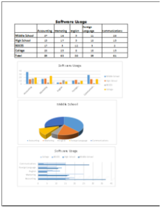
Completed Assignment

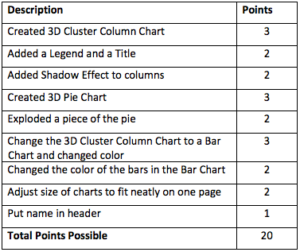
Check the rubric below to be sure you have completed all the tasks.


