
5.2: 3-D Reference Sheet – Information and Practice
- Page ID
- 13035
\( \newcommand{\vecs}[1]{\overset { \scriptstyle \rightharpoonup} {\mathbf{#1}} } \)
\( \newcommand{\vecd}[1]{\overset{-\!-\!\rightharpoonup}{\vphantom{a}\smash {#1}}} \)
\( \newcommand{\dsum}{\displaystyle\sum\limits} \)
\( \newcommand{\dint}{\displaystyle\int\limits} \)
\( \newcommand{\dlim}{\displaystyle\lim\limits} \)
\( \newcommand{\id}{\mathrm{id}}\) \( \newcommand{\Span}{\mathrm{span}}\)
( \newcommand{\kernel}{\mathrm{null}\,}\) \( \newcommand{\range}{\mathrm{range}\,}\)
\( \newcommand{\RealPart}{\mathrm{Re}}\) \( \newcommand{\ImaginaryPart}{\mathrm{Im}}\)
\( \newcommand{\Argument}{\mathrm{Arg}}\) \( \newcommand{\norm}[1]{\| #1 \|}\)
\( \newcommand{\inner}[2]{\langle #1, #2 \rangle}\)
\( \newcommand{\Span}{\mathrm{span}}\)
\( \newcommand{\id}{\mathrm{id}}\)
\( \newcommand{\Span}{\mathrm{span}}\)
\( \newcommand{\kernel}{\mathrm{null}\,}\)
\( \newcommand{\range}{\mathrm{range}\,}\)
\( \newcommand{\RealPart}{\mathrm{Re}}\)
\( \newcommand{\ImaginaryPart}{\mathrm{Im}}\)
\( \newcommand{\Argument}{\mathrm{Arg}}\)
\( \newcommand{\norm}[1]{\| #1 \|}\)
\( \newcommand{\inner}[2]{\langle #1, #2 \rangle}\)
\( \newcommand{\Span}{\mathrm{span}}\) \( \newcommand{\AA}{\unicode[.8,0]{x212B}}\)
\( \newcommand{\vectorA}[1]{\vec{#1}} % arrow\)
\( \newcommand{\vectorAt}[1]{\vec{\text{#1}}} % arrow\)
\( \newcommand{\vectorB}[1]{\overset { \scriptstyle \rightharpoonup} {\mathbf{#1}} } \)
\( \newcommand{\vectorC}[1]{\textbf{#1}} \)
\( \newcommand{\vectorD}[1]{\overrightarrow{#1}} \)
\( \newcommand{\vectorDt}[1]{\overrightarrow{\text{#1}}} \)
\( \newcommand{\vectE}[1]{\overset{-\!-\!\rightharpoonup}{\vphantom{a}\smash{\mathbf {#1}}}} \)
\( \newcommand{\vecs}[1]{\overset { \scriptstyle \rightharpoonup} {\mathbf{#1}} } \)
\(\newcommand{\longvect}{\overrightarrow}\)
\( \newcommand{\vecd}[1]{\overset{-\!-\!\rightharpoonup}{\vphantom{a}\smash {#1}}} \)
\(\newcommand{\avec}{\mathbf a}\) \(\newcommand{\bvec}{\mathbf b}\) \(\newcommand{\cvec}{\mathbf c}\) \(\newcommand{\dvec}{\mathbf d}\) \(\newcommand{\dtil}{\widetilde{\mathbf d}}\) \(\newcommand{\evec}{\mathbf e}\) \(\newcommand{\fvec}{\mathbf f}\) \(\newcommand{\nvec}{\mathbf n}\) \(\newcommand{\pvec}{\mathbf p}\) \(\newcommand{\qvec}{\mathbf q}\) \(\newcommand{\svec}{\mathbf s}\) \(\newcommand{\tvec}{\mathbf t}\) \(\newcommand{\uvec}{\mathbf u}\) \(\newcommand{\vvec}{\mathbf v}\) \(\newcommand{\wvec}{\mathbf w}\) \(\newcommand{\xvec}{\mathbf x}\) \(\newcommand{\yvec}{\mathbf y}\) \(\newcommand{\zvec}{\mathbf z}\) \(\newcommand{\rvec}{\mathbf r}\) \(\newcommand{\mvec}{\mathbf m}\) \(\newcommand{\zerovec}{\mathbf 0}\) \(\newcommand{\onevec}{\mathbf 1}\) \(\newcommand{\real}{\mathbb R}\) \(\newcommand{\twovec}[2]{\left[\begin{array}{r}#1 \\ #2 \end{array}\right]}\) \(\newcommand{\ctwovec}[2]{\left[\begin{array}{c}#1 \\ #2 \end{array}\right]}\) \(\newcommand{\threevec}[3]{\left[\begin{array}{r}#1 \\ #2 \\ #3 \end{array}\right]}\) \(\newcommand{\cthreevec}[3]{\left[\begin{array}{c}#1 \\ #2 \\ #3 \end{array}\right]}\) \(\newcommand{\fourvec}[4]{\left[\begin{array}{r}#1 \\ #2 \\ #3 \\ #4 \end{array}\right]}\) \(\newcommand{\cfourvec}[4]{\left[\begin{array}{c}#1 \\ #2 \\ #3 \\ #4 \end{array}\right]}\) \(\newcommand{\fivevec}[5]{\left[\begin{array}{r}#1 \\ #2 \\ #3 \\ #4 \\ #5 \\ \end{array}\right]}\) \(\newcommand{\cfivevec}[5]{\left[\begin{array}{c}#1 \\ #2 \\ #3 \\ #4 \\ #5 \\ \end{array}\right]}\) \(\newcommand{\mattwo}[4]{\left[\begin{array}{rr}#1 \amp #2 \\ #3 \amp #4 \\ \end{array}\right]}\) \(\newcommand{\laspan}[1]{\text{Span}\{#1\}}\) \(\newcommand{\bcal}{\cal B}\) \(\newcommand{\ccal}{\cal C}\) \(\newcommand{\scal}{\cal S}\) \(\newcommand{\wcal}{\cal W}\) \(\newcommand{\ecal}{\cal E}\) \(\newcommand{\coords}[2]{\left\{#1\right\}_{#2}}\) \(\newcommand{\gray}[1]{\color{gray}{#1}}\) \(\newcommand{\lgray}[1]{\color{lightgray}{#1}}\) \(\newcommand{\rank}{\operatorname{rank}}\) \(\newcommand{\row}{\text{Row}}\) \(\newcommand{\col}{\text{Col}}\) \(\renewcommand{\row}{\text{Row}}\) \(\newcommand{\nul}{\text{Nul}}\) \(\newcommand{\var}{\text{Var}}\) \(\newcommand{\corr}{\text{corr}}\) \(\newcommand{\len}[1]{\left|#1\right|}\) \(\newcommand{\bbar}{\overline{\bvec}}\) \(\newcommand{\bhat}{\widehat{\bvec}}\) \(\newcommand{\bperp}{\bvec^\perp}\) \(\newcommand{\xhat}{\widehat{\xvec}}\) \(\newcommand{\vhat}{\widehat{\vvec}}\) \(\newcommand{\uhat}{\widehat{\uvec}}\) \(\newcommand{\what}{\widehat{\wvec}}\) \(\newcommand{\Sighat}{\widehat{\Sigma}}\) \(\newcommand{\lt}{<}\) \(\newcommand{\gt}{>}\) \(\newcommand{\amp}{&}\) \(\definecolor{fillinmathshade}{gray}{0.9}\)What are sheets?
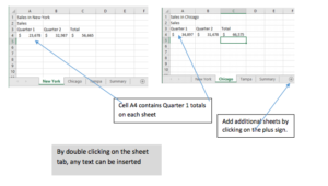
Sheets are separate, individual spreadsheets. To access sheets, look at the bottom of the screen of a spreadsheet and notice the tab called “Sheets.” A “workbook” is comprised of any number of sheets. Sheets can be added by clicking the plus sign next to the tab “sheets.”
Sheet tabs can be changed from the word “sheets” to any label. To change a name on a sheet, double click the sheet tab and insert a new label name.
In the example below, a company has business in several cities. Each city has a separate sheet in a workbook. The sheets have been renamed New York, Chicago, Tampa and Summary. Each sheet has the same format, that is each sheet is set up with the same cell references. Notice that Quarter 1 sales for New York is in cell A4; Quarter 1 sales for Chicago and Tampa are also in A4 on that sheet.
What is 3-D referencing?
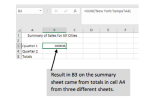
The 3-D referencing is used to summarize specific information on each of the sheets and place the total on a separate summary page.
For example, in the illustration above, the total of Quarter 1 in cell A4 for each of the cities can be quickly summarized and placed on the Summary sheet in a different position such as B3.
It would look like this:
How do I develop the formula?
When summarizing data, you are actually adding. The SUM formula works well for a 3-D referencing exercise. In a regular worksheet when one adds multiply columns, a range is selected. When AutoSum is used, that automatically references a range of numbers. If AutoSum is not used, a range of numbers can be selected by highlighting the column or row to add. In both the AutoSum feature or using the SUM feature, the formula shows a colon between the first and the last cell reference. For example, =SUM(B4:B10) would add up rows 4 through 10 in column B.
The part that is different is 3-D referencing is incorporating the different sheets. To get the Quarter 1 Sales for three different cities- New York, Chicago, and Tampa – (in the example above), start by placing your mouse cursor in the cell of the Summary sheet where you want the result to show. In the example above, I put my mouse cursor in B3. It doesn’t matter what cell, but you do have to start on the Summary Sheet. Then follow the next steps.
1. Type the equal sign followed by the word SUM and an open parenthesis.
2. Click the first city sheet (New York). Hold down the SHIFT key and click the last city (Tampa). In the formula, you will notice that the colon was placed automatically between New York and Tampa which would also include Chicago.
3. Next click the cell reference on the New York, or first sheet, that contains the amount you want to total. In this case, click on A4.
4. Enter.
5. The total (100698) appears on the Summary Sheet in cell B3 where you started the formula.
6. The formula displays in the formula bar above the worksheet.
The formula is =SUM(‘New York:Tampa’!A4)
7. Notice the exclamation point before the cell reference. This indicates a 3-D Reference. The apostrophes automatically appear when a 3-D reference is used.
PRACTICE EXERCISE: (This isn’t graded, but you might find it useful for understanding 3-D Referencing.)
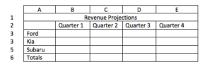
1. Create a spreadsheet using the information below. Merge and Center the title.
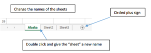
2. At the bottom of the screen, double-click on the tab “Sheet 1” and type Alaska. This spread sheet will be used for Alaska. Please see illustration below Step 5.
3. Next click the circled plus sign at the very bottom of the window next to the tab “Sheet” and create a “Sheet 2”. Name this sheet Arkansas.
4. Once again click the plus sign at the bottom for “Sheet 3” and name that sheet Alabama.
5. Finally click the plus sign again for “Sheet 4” and name it Summary.
6. Click on the Alaska tab.
7. On the sheet for Alaska, insert a SUM formula to add the total for Quarter 1. Although there are no amounts at this time, you can insert a formula which will compute totals after you put in the figures. A zero will show for now indicating there is a formula in that cell.
8. Using AutoFill, pull the formula from B6 to E6.
9. After the formula has been inserted, select A1 to E6. Release the mouse then right click on the selected columns and rows. From the short cut menu that displays, click COPY. (You can also select A1 to E6 and click on COPY from the HOME tab, Clipboard Group.)
10. Click Arkansas tab then click in cell A1.
11. Click paste (either from the short cut menu or from the ribbon). An exact duplicate of information on the Alaska sheet including a SUM formula is now on the Arkansas sheet.
12. Follow steps 7 to Step 9 to paste the formatted table to the Alabama sheet.
13. Next, insert different amounts in the four Quarters for the three different car types on ALL three sheets. As you put the amounts in, notice that you are also getting a total for the columns.
14. Next click on the Summary sheet tab.
15. In cell A3 on the Summary sheet, type “Ford.” In cell A4 type “Kia.” In cell A5 type “Subaru.” In cell A6 type “Total.” (See the illustration below.)
16. In cell A1 give this table a title: “Summary 4th Quarter Total Sales.”
17. Use the merge and center feature to center the title over the table between columns A to D.
18. In cell B 2, type the heading “Quarter 4”.
19. Create a 3-D Reference formula by clicking in cell B3. Start with an equal sign followed by the word SUM. (=SUM). See the instructions for 3D formulas on the 3-D Reference Sheets Information Step 1.
20. Follow Steps 2-6 to create a 3D Referencing formula.
21. The formula and summary sheet should look like this one: (although the total will be different depending on the amounts inputted for each city
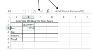
16. Once the formula in B3 on the SUMMARY sheet is inserted, use the AutoFill to pulled down the 3D Referencing formula from B3 to B6. Notice that the formula cell reference changed for each city but the rest of the formula stated the same. You have completed a 3D Referencing exercise!
- 3-D Reference Sheet u2013 Information and Practice. Authored by: Fran Wells. License: CC BY: Attribution