7.2: Spreadsheets to Estimate Costs

Learning Objectives

• Format a spreadsheet to make it more readable and professional in appearance.
• Create an assumptions area
• Name cells in a spreadsheet
• Use spreadsheet names in formulas
• Insert rows and columns into a spreadsheet.
• Perform a sensitivity analysis
• Apply graphic design principles to create professional looking spreadsheets.

Apply the C.R.A.P. Principles

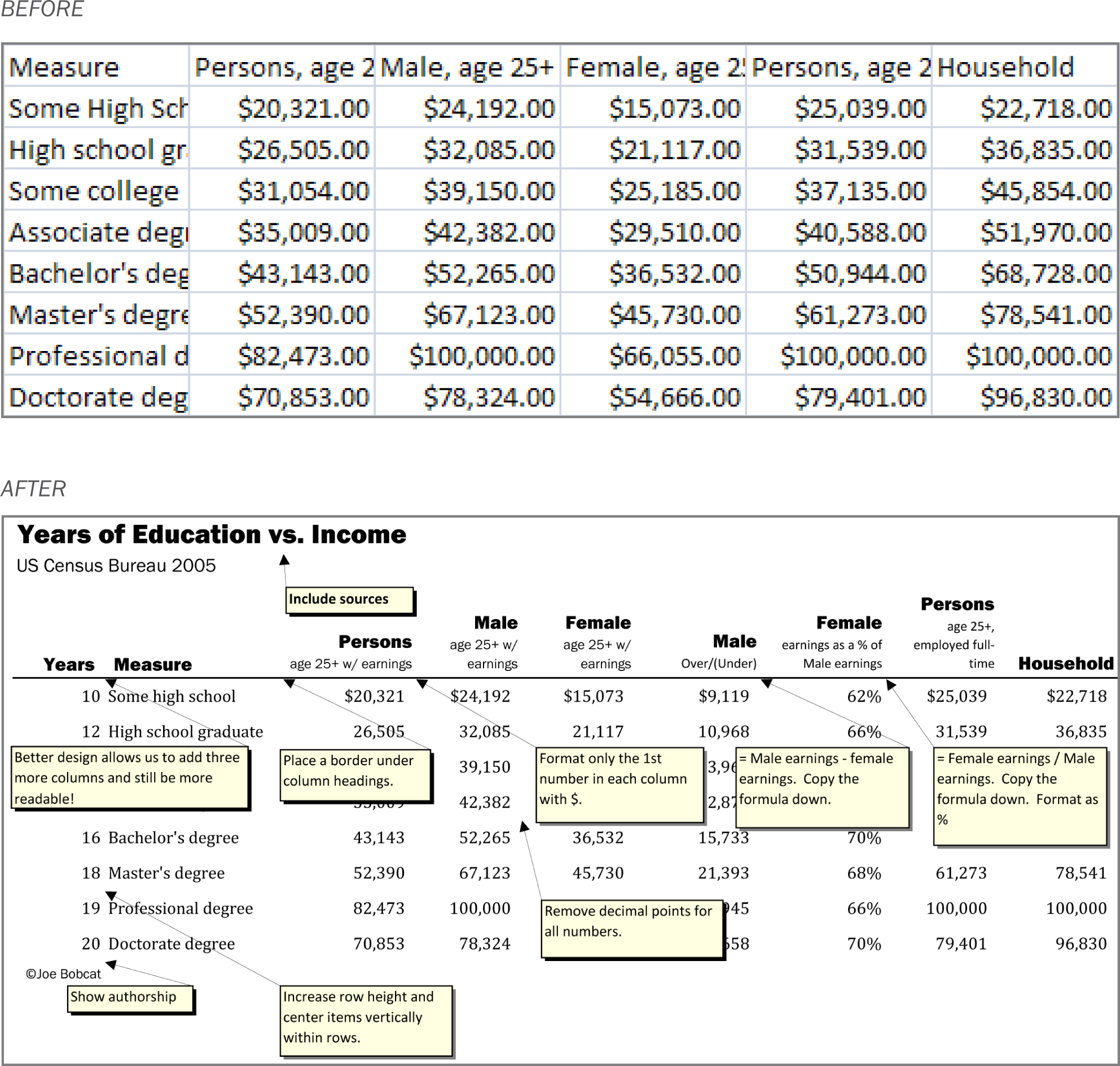
Notice the spreadsheets on the following page. The “before” spreadsheet is both sloppy and hard to read. The “after” spreadsheet uses contrast in fonts and size to focus attention on important information, and it uses alignment to create strength and clarity. Numbers and their headings are right justified, and the “Measure” category and its heading is left justified. Proximity and repetition of fonts create a professional finished look.

The “after” spreadsheet also includes three new columns: Years, Male Over/(Under), and Female earnings as a % of male earnings. These new columns are processed data or information. Information summarizes or describes the data in a meaningful way. This information shows that disparity between male and female earnings both as an absolute value and as a percentage. To create information usually involves a formula. Formulas are written by the user to perform calculations on data. Business formulas tend to be simple, usually involving addition, subtraction, multiplication, or division. For example Male Over/(Under) subtracts female earnings from male earnings to show the difference between the two. Similarly female earnings as a percentage of male earnings divides female earnings by male earnings. Note that the information revealed by these columns tells us that there is a difference; it does not tell us why. And most information is very much like this. It needs to be interpreted in order to make business decisions, or in this case public policy decisions.

The total area of a spreadsheet often exceeds the normal width of printing paper. Address this problem by printing in landscape orientation and by scaling the page to the width of the paper.

Formatting a spreadsheet makes an enormous difference as to its professionalism. Proper formatting also makes the data much more readable.

Place Estimates in an Assumptions Area

We mentioned previously that all forecasting involves making assumptions. These are educated guesses based upon research. However, assumptions may change over time. Ideally, you would like to be able to update your spreadsheet easily as the assumptions change. The easiest and most error free way to perform the updates is to use an assumptions area.

An assumptions area contains all of the variables that go into your calculations. It is normally located at the top of the spreadsheet. In a perfectly designed spreadsheet, the assumptions area is the only place that you actually type a number. Every other cell in the spreadsheet is a formula that refers back directly or indirectly to the assumptions area.

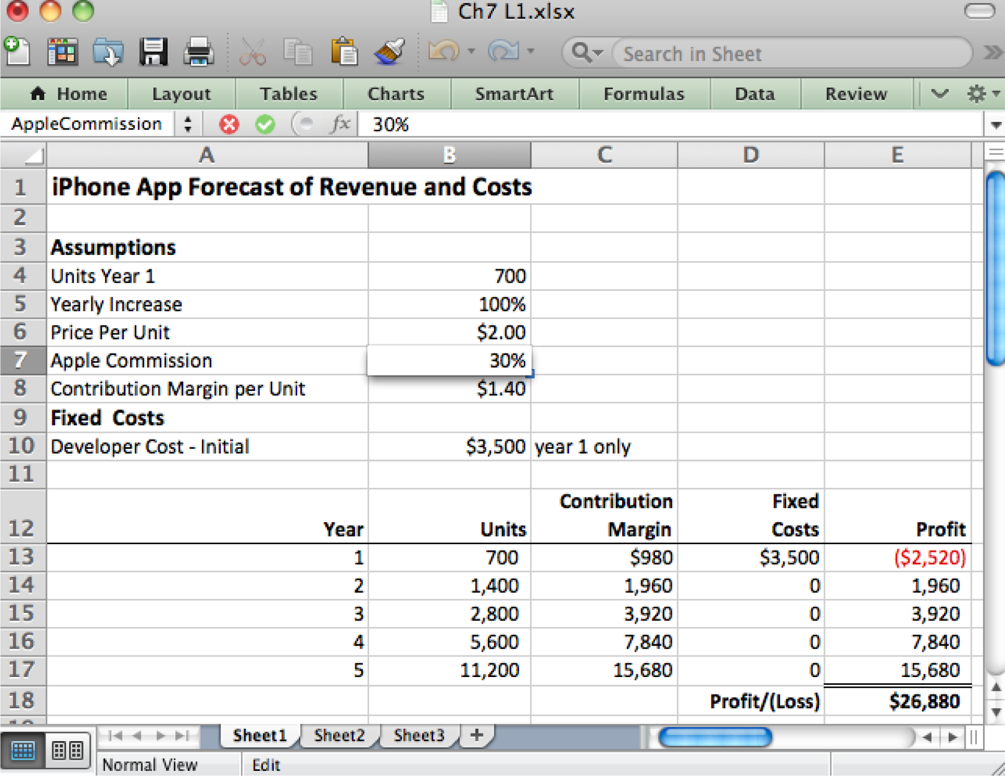
Consider the Apple Commission located in cell B7. We need to know the commission in order to calculate the contribution margin—how much we make on each sale. We would expect the contribution margin formula in B8 to reference B7. So the formula in B8 might look like this:

=B6*(1-B7)

However, that formula is not particularly informative. The problem is that Excel does not know the meaning of the numbers in B7 and B8. It does not examine the labels to the left either. If we gave cells B6 and B7 meaningful names, we could calculate contribution margin as:

=PricePerUnit*(1-AppleCommission)

or equivalently

=PricePerUnit-(PricePerUnit*AppleCommission)

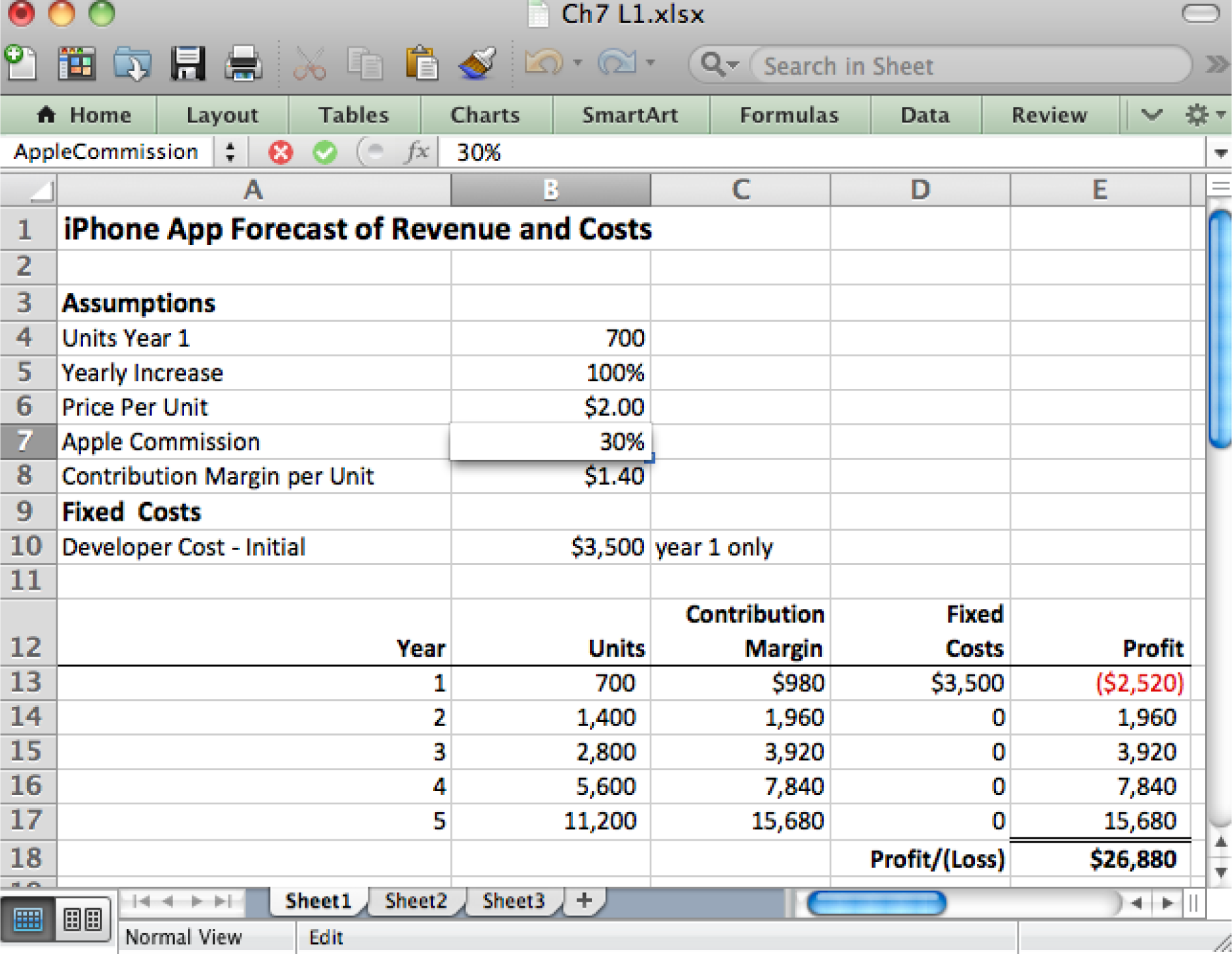
Note how these names are very similar to the labels. We say very similar because cell names can not contain spaces, whereas labels can. The cell names will be hidden from view but can be used in calculations as shown above.

The place where you create the names is in the name box on the toolbar just above cell A1. Simply type the name and hit Enter. You must hit Enter or the name will not stick.

Remember cell names can not contain spaces. So “Apple_Commission” is OK and so is “AppleCommission.” However, “Apple Commission” as two words with a space in between will not work. By the way, capitalizing the first letter of each word and eliminating the spaces between words (e.g., PricePerUnit) is called CamelBack notation for obvious reasons.

In a well designed spreadsheet the only place that numbers should be updated is in the assumptions area. Every other cell references the assumptions area using formulas.

Formulas are Used to Generate Information

Our last example showed a formula in the assumptions area. It is rare to have formulas in the assumptions area. Most formulas appear in the spreadsheet proper below the assumptions area.

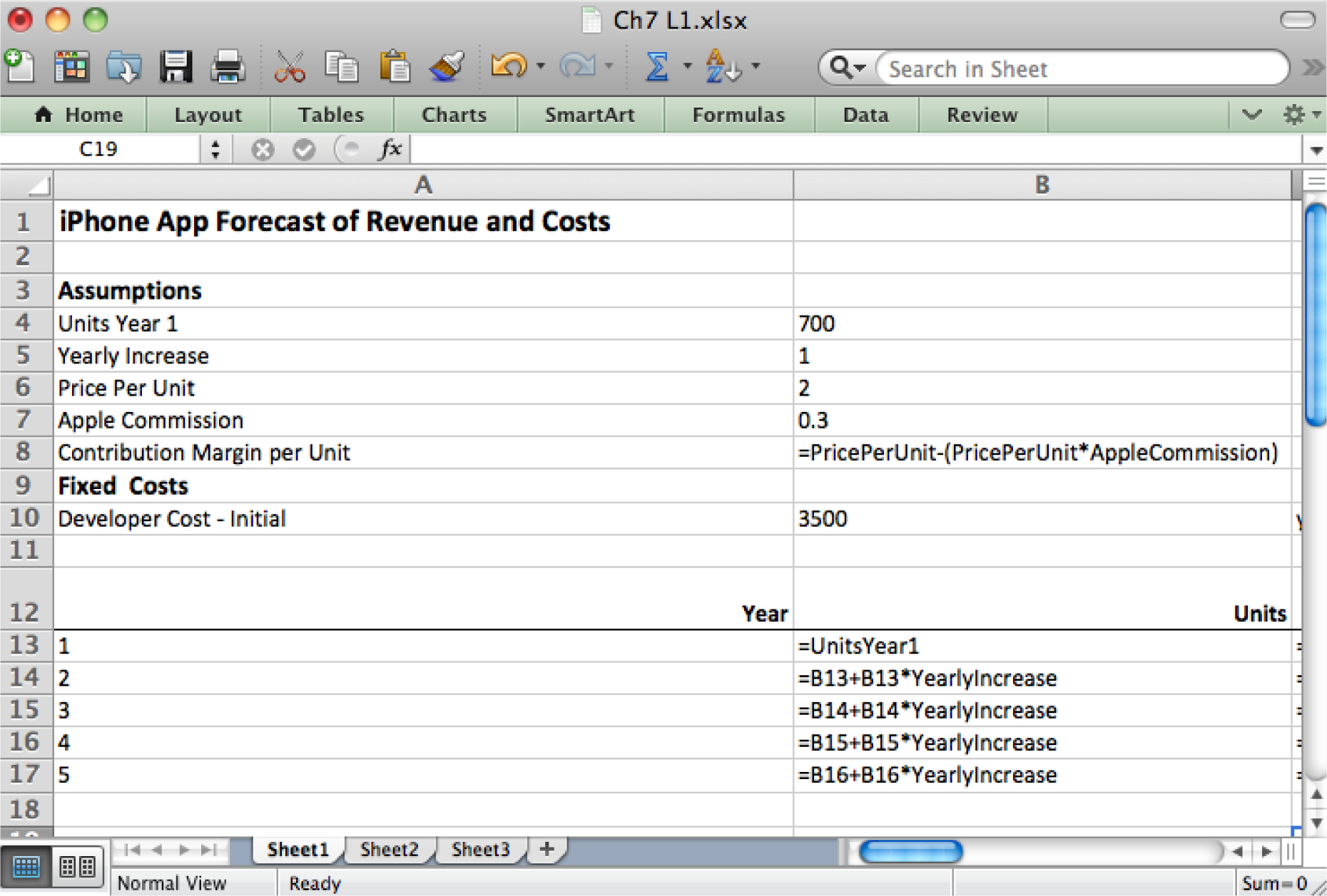
Let us assume that we named B4 as UnitsYear1. Then the formula in B13 is =UnitsYear1. Every formula begins with an equal sign.

B14 is a much more interesting example, and one that shows the power of Excel. We are now in Year 2 and need to represent the projected increase in sales. To represent any increase involves taking the prior value (B13) and adding the increase to it. Calculate the increase by multiplying the prior value by the percentage increase. So we get:

=B13+B13*YearlyIncrease (700+700*100%)

The first B12 is the prior value; the second B12*YearlyIncrease is the amount of the increase. The great thing about this formula is that it can be copied down to the rest of the cells in column B. Simply double click or drag the bottom right corner of B13 and the rest of the column will fill as follows:

B15: =B14+B14*YearlyIncrease (1400+1400*100%)

B16: =B15+B15*YearlyIncrease (2800+2800*100%)

B17: =B16+B16*YearlyIncrease (5600+5600*100%)

Excel properly repeats the pattern without any further effort on your part! However, note carefully that this was only possible because we had earlier named B5 as YearlyIncrease. If we do not name B5 then the pattern would look like this:

B14: =B13+B13*B5 CORRECT (700+700*100%)

B15: =B14+B14*B6 WRONG (1400+1400*$2.00)

B16: =B15+B15*B7 WRONG (3200+3200*30%)

B17: =B16+B16*B8 WRONG (5440+5440*$1.40)

Excel improperly repeats the pattern moving every cell down one space each time. That is a problem for B5 in the assumptions area because the next cells down are Price Per Unit (B6=$2.00), Apple Commission (B7=30%), and Contribution Margin per Unit (B8=$1.40). These last three have nothing to do with units sold and we get gibberish instead of valuable information. What is even more frightening is that the numbers do not look obviously wrong.

So in addition to being more readable, naming cells in the assumptions area also protects us against errors when copying formulas.

Above each cell in the assumptions area gets a unique name. For example, B7 is called AppleCommission (with no spaces allowed in the name). Below formulas in the calculation section reference values in the assumptions area by name. For example, the formula in B13 references the YearlyIncrease field. Such formulas may be copied down the column without fear that the formula will improperly change when copied.

Perform a Sensitivity Analysis to Hedge Your Bets

Any time you make assumptions, you have to allow for the possibility that you might be wrong. Since you are dealing with real money, some of which is probably yours or a relative’s, you need to know the extent of your exposure should things not work out as planned.

Therefore, it is a good idea to vary the assumptions and see what outcomes occur. This sophisticated analysis allows you to have an intelligent discussion about possible future scenarios.

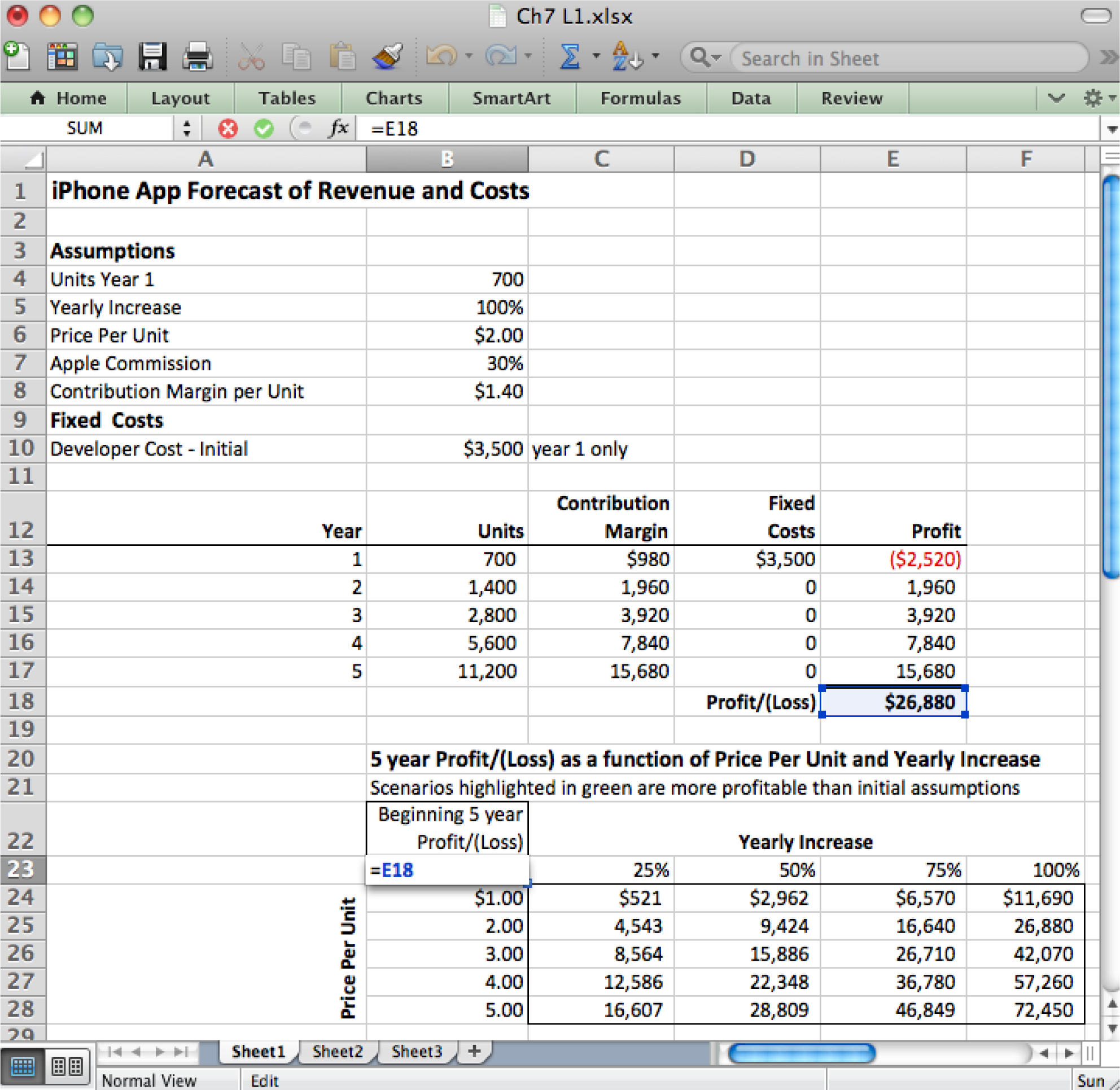
A good way to conduct a sensitivity analysis is using an Excel data table. A table can represent three variables—column headings, row headings, and the results inside the table. You vary the data in the row and column headings to observe changes inside the table. For example, assume that each cell inside the table contains the profit after Year 5. We can vary the growth rate and price per unit to see the effect on profit.

To perform these calculations without the data table would require manually changing growth rate and price per unit assumptions TWENTY times and recording the values after year 5—this is busy work. By contrast, Excel has the built in ability to create a data table.

The trickiest part of creating a data table is shown by the highlighted cells in the spreadsheet. You must repeat the value from your calculations on which you wish to perform the analysis. And not only do you have to repeat it, but you must repeat it using a simple formula. So the formula in B23 is:

B23: =E18

Note how this cell must form the upper left corner of the data table. Now just fill in the row and column headings. We put various values for growth rate in the column headings and various values for price per unit in the row headings. Next highlight the whole table including the row and column headings and choose What If Analysis > Data Table. The last step is to identify for Excel the first cells where growth rate and price per unit appear in the assumptions area. Then Excel will substitute the values from the row and column headings into the assumptions area, redo ALL the calculations in the spreadsheet and then capture the results in the data table—all behind the scenes!

Now it is your job to argue for the ones you think are most favorable and realistic.

Key Takeaways

• Well designed spreadsheets group input variables into an assumptions area. Ideally, the assumptions area is the only place that numbers are typed.
• Formulas may be copied. However, cells that should not change in a formula should be named.
• Many information systems projects fail. Your exposure can be analyzed in a sensitivity analysis using a data table.

Questions and Exercises

1. Without using the built in data table function, how could you still construct a table that would perform a sensitivity analysis.

Make sure that the upper left corner of the data table is a simple formula that copies the value that you want to see varied in the data table.

Techniques

The following techniques, found in the PowerPoint section of the software reference, may be useful in completing the assignments for this chapter: Overview Map of Interface • Cell Name-Create • Cell Name-Delete • Format Number • Formula-Copy • Formula-Create • Formula Mode • Insert Column • Insert Row • Move Decimal Point • Sensitivity Analysis

L1 Assignment: Forecast Revenues/Expenses

Professionals are able to represent what they know intuitively in a properly formatted spreadsheet with an assumptions area.

Setup

Start Excel and properly title your spreadsheet.

Content and Style

• Create an assumptions area containing all variables.
• Name each number in the assumptions area.
• Use those names in calculations in the spreadsheet below. Except for the Year column, EVERY number outside of the Assumptions area must be calculated with formulas.
• Follow best practice design techniques in this chapter.
• Only the first number in each column gets formatted as CURRENCY (Do not format as ACCOUNTING.) Update the format using the Number Formatting Technique. All other numbers greater than 1,000 should be in Comma style.
• Include a copyright symbol with your name at the bottom.
• The worksheet gridlines will not appear on the printout.

Deliverables

Electronic submission: Submit the workbook electronically.

Paper submission:

• Print out both the results and formulas. The formulas printout shows the formulas in each column. Reveal the formulas by typing CTRL+ ~ (press the CTRL and ~ keys at the same time). Adjust the column widths to closely crop the formulas by dragging the separator between each column in the gray header area.
• Both printouts should use landscape orientation, which you will find under Page Layout > Page Setup > Orientation > Landscape. Each printout should fit on one page. Choose Page Layout > Scale to Fit > Height: 1 page; Width: 1 page.

Please save the forecast revenues/costs spreadsheet; you will be updating it later.

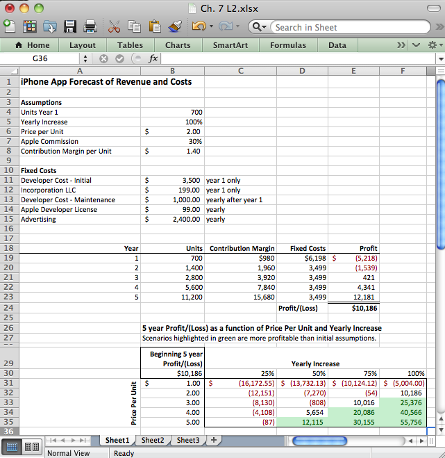
L2 Assignment: More Expenses and Sensitivity Analysis

To make the problem more realistic, we bring in additional fixed costs. To help in decision making, we perform a sensitivity analysis.

Setup

Re-save your workbook file from the L1 under a new name and then modify it to look as below. This must be a new workbook—do not simply create a new sheet in the same workbook or some of your names will conflict and spoil the data table.

Content and Style

• Incorporate new costs including Incorporation ($199), Apple Developer Cost ($99/year), Advertising ($2,400/yr.), Developer maintenance cost ($1,000/yr.). Create an assumptions area containing all variables.
• Name each number in the assumptions area.
• Use those names in calculations in the spreadsheet below. Except for the Year column, EVERY number outside of the assumptions area must be calculated with formulas.
• Follow best practice design techniques in this chapter.
• Only the first number in each column gets formatted as CURRENCY. (Do not format as ACCOUNTING.) Update the format using the Number Formatting Technique. All other numbers greater than 1,000 should be in Comma style.
• Include a copyright symbol with your name at the bottom.
• The worksheet gridlines will not appear on the printout.
• Produce a sensitivity analysis table of total profit/(loss) as a function of growth rate and price per unit.

Deliverables

Electronic submission: Submit the workbook electronically.

Paper submission:

• Print out both the results and formulas. The formulas printout shows the formulas in each column. Reveal the formulas by typing CTRL+ ~. Adjust the column widths to closely crop the formulas by dragging the separator between each column in the gray header area.
• Both printouts should use landscape orientation, which you will find under Page Layout > Page Setup > Orientation > Landscape. Each printout should fit on one page. Choose Page Layout > Scale to Fit > Height: 1 page; Width: 1 page.

Add assumptions and columns as necessary to accommodate additional costs of maintenance, incorporation, and advertising.